📖 Comprehensive Guide to evanverse
Welcome to the comprehensive guide for evanverse - a feature-rich R utility package providing 55+ functions for data analysis, visualization, and bioinformatics workflows.
🚀 Package Installation and Setup
# Install from CRAN
install.packages("evanverse")

# Or install development version from GitHub
evanverse::inst_pkg("evanbio/evanverse")📦 Package Management
The evanverse package provides robust package management utilities:
# Check if packages are installed
required_packages <- c("dplyr", "ggplot2", "tidyr")
check_pkg(required_packages)
#> # A tibble: 3 × 4
#>   package name    installed source
#>   <chr>   <chr>   <lgl>     <chr>
#> 1 dplyr   dplyr   TRUE      CRAN
#> 2 ggplot2 ggplot2 TRUE      CRAN
#> 3 tidyr   tidyr   TRUE      CRAN

# Get package version (skip on CRAN due to network dependency)
if (!identical(Sys.getenv("NOT_CRAN"), "false")) {
  try(pkg_version("evanverse"), silent = TRUE)
}
#>     package version latest source
#> 1 evanverse   0.4.4  0.4.0   CRAN
🎨 Color Palette System
Available Palettes
# List all available palettes
palettes_info <- list_palettes()
print(palettes_info)
#> name type n_color
#> 12 div_contrast diverging 2
#> 14 div_fireice diverging 2
#> 16 div_polar diverging 2
#> 18 div_sunset diverging 2
#> 15 div_pinkgreen_rb diverging 3
#> 13 div_earthy diverging 5
#> 17 div_sage diverging 7
#> 29 qual_earthy qualitative 3
#> 70 qual_primary qualitative 3
#> 77 qual_softtrio qualitative 3
#> 90 qual_vintage qualitative 3
#> 21 qual_balanced qualitative 4
#> 30 qual_egypt_met qualitative 4
#> 46 qual_kandinsky_met qualitative 4
#> 34 qual_greek_met qualitative 5
#> 40 qual_isfahan2_met qualitative 5
#> 42 qual_java_met qualitative 5
#> 44 qual_johnson_met qualitative 5
#> 56 qual_navajo_met qualitative 5
#> 58 qual_newkingdom_met qualitative 5
#> 79 qual_tara_met qualitative 5
#> 89 qual_vibrant qualitative 5
#> 91 qual_violin qualitative 5
#> 93 qual_wissing_met qualitative 5
#> 33 qual_gauguin_met qualitative 6
#> 35 qual_harmony qualitative 6
#> 38 qual_homer2_met qualitative 6
#> 45 qual_juarez_met qualitative 6
#> 47 qual_klimt_met qualitative 6
#> 48 qual_lakota_met qualitative 6
#> 64 qual_pastel qualitative 6
#> 66 qual_peru1_met qualitative 6
#> 67 qual_peru2_met qualitative 6
#> 68 qual_pillement_met qualitative 6
#> 19 qual_archambault_met qualitative 7
#> 20 qual_austria_met qualitative 7
#> 26 qual_degas_met qualitative 7
#> 28 qual_derain_met qualitative 7
#> 36 qual_hokusai1_met qualitative 7
#> 41 qual_jama_g qualitative 7
#> 53 qual_moreau_met qualitative 7
#> 55 qual_nattier_met qualitative 7
#> 62 qual_okeeffe2_met qualitative 7
#> 69 qual_pissaro_met qualitative 7
#> 82 qual_tron_g qualitative 7
#> 84 qual_tsimshian_met qualitative 7
#> 85 qual_vangogh1_met qualitative 7
#> 88 qual_veronese_met qualitative 7
#> 22 qual_cassatt1_met qualitative 8
#> 37 qual_homer1_met qualitative 8
#> 39 qual_ingres_met qualitative 8
#> 54 qual_morgenstern_met qualitative 8
#> 57 qual_nejm_g qualitative 8
#> 59 qual_nizami_met qualitative 8
#> 74 qual_set2_rb qualitative 8
#> 78 qual_tam_met qualitative 8
#> 80 qual_thomas_met qualitative 8
#> 81 qual_tiepolo_met qualitative 8
#> 83 qual_troy_met qualitative 8
#> 86 qual_vangogh2_met qualitative 8
#> 87 qual_vangogh3_met qualitative 8
#> 25 qual_cross_met qualitative 9
#> 49 qual_lancet_g qualitative 9
#> 52 qual_monet_met qualitative 9
#> 73 qual_set1_rb qualitative 9
#> 92 qual_vivid qualitative 9
#> 23 qual_cassatt2_met qualitative 10
#> 24 qual_cosmic_g qualitative 10
#> 27 qual_demuth_met qualitative 10
#> 31 qual_flatui_g qualitative 10
#> 43 qual_jco_g qualitative 10
#> 51 qual_mobility qualitative 10
#> 60 qual_npg_g qualitative 10
#> 50 qual_manet_met qualitative 11
#> 61 qual_okeeffe1_met qualitative 11
#> 63 qual_paquin_met qualitative 11
#> 32 qual_futurama_g qualitative 12
#> 71 qual_redon_met qualitative 12
#> 72 qual_renoir_met qualitative 12
#> 75 qual_set3_rb qualitative 12
#> 76 qual_signac_met qualitative 14
#> 65 qual_pbmc_sc qualitative 17
#> 2 seq_blues sequential 3
#> 3 seq_blush sequential 4
#> 4 seq_forest sequential 4
#> 11 seq_muted sequential 4
#> 6 seq_hokusai2 sequential 6
#> 7 seq_hokusai3 sequential 6
#> 9 seq_locuszoom sequential 7
#> 8 seq_isfahan sequential 8
#> 10 seq_mobility sequential 9
#> 5 seq_hiroshige sequential 10
#> 1 seq_benedictus sequential 13
#> colors
#> 12 #C64328, #56BBA5
#> 14 #2AA6C6, #C64328
#> 16 #8CB5D2, #E18E8F
#> 18 #57A2FF, #FF8000
#> 15 #E64B35B2, #00A087B2, #3C5488B2
#> 13 #283618, #606C38, #FEFAE0, #DDA15E, #BC6C25
#> 17 #EDEAE7, #B1CABA, #BBCDD7, #BBAAB6, #6D8092, #504B54, #0E0F0F
#> 29 #C64328, #56BBA5, #E3A727
#> 70 #C64328, #2AA6C6, #E3A727
#> 77 #E64B35B2, #00A087B2, #3C5488B2
#> 90 #96A0D9, #D9BDAD, #D9D5A0
#> 21 #5D83B4, #9FD0E8, #CDAE9D, #959683
#> 30 #dd5129, #0f7ba2, #43b284, #fab255
#> 46 #3b7c70, #ce9642, #898e9f, #3b3a3e
#> 34 #3c0d03, #8d1c06, #e67424, #ed9b49, #f5c34d
#> 40 #d7aca1, #ddc000, #79ad41, #34b6c6, #4063a3
#> 42 #663171, #cf3a36, #ea7428, #e2998a, #0c7156
#> 44 #a00e00, #d04e00, #f6c200, #0086a8, #132b69
#> 56 #660d20, #e59a52, #edce79, #094568, #e1c59a
#> 58 #e1846c, #9eb4e0, #e6bb9e, #9c6849, #735852
#> 79 #eab1c6, #d35e17, #e18a1f, #e9b109, #829d44
#> 89 #BF3F9D, #B3BCD7, #6DA6A0, #D98A29, #F2C894
#> 91 #37848C, #F2935C, #F2A88D, #D95555, #A7CAE9
#> 93 #4b1d0d, #7c291e, #ba7233, #3a4421, #2d5380
#> 33 #b04948, #811e18, #9e4013, #c88a2c, #4c6216, #1a472a
#> 35 #BF3641, #836AA6, #377BA6, #448C42, #D96236, #B79290
#> 38 #bf3626, #e9851d, #f9c53b, #aeac4c, #788f33, #165d43
#> 45 #a82203, #208cc0, #f1af3a, #cf5e4e, #637b31, #003967
#> 47 #df9ed4, #c93f55, #eacc62, #469d76, #3c4b99, #924099
#> 48 #04a3bd, #f0be3d, #931e18, #da7901, #247d3f, #20235b
#> 64 #B2AA76, #8C91CF, #D7D79C, #DABFAC, #BCEDDB, #C380A0
#> 66 #b5361c, #e35e28, #1c9d7c, #31c7ba, #369cc9, #3a507f
#> 67 #65150b, #961f1f, #c0431f, #f19425, #c59349, #533d14
#> 68 #a9845b, #697852, #738e8e, #44636f, #2b4655, #0f252f
#> 19 #88a0dc, #381a61, #7c4b73, #ed968c, #ab3329, #e78429, #f9d14a
#> 20 #a40000, #16317d, #007e2f, #ffcd12, #b86092, #721b3e, #00b7a7
#> 26 #591d06, #96410e, #e5a335, #556219, #418979, #2b614e, #053c29
#> 28 #efc86e, #97c684, #6f9969, #aab5d5, #808fe1, #5c66a8, #454a74
#> 36 #6d2f20, #b75347, #df7e66, #e09351, #edc775, #94b594, #224b5e
#> 41 #374E55, #DF8F44, #00A1D5, #B24745, #79AF97, #6A6599, #80796B
#> 53 #421600, #792504, #bc7524, #8dadca, #527baa, #104839, #082844
#> 55 #52271c, #944839, #c08e39, #7f793c, #565c33, #184948, #022a2a
#> 62 #fbe3c2, #f2c88f, #ecb27d, #e69c6b, #d37750, #b9563f, #92351e
#> 69 #134130, #4c825d, #8cae9e, #8dc7dc, #508ca7, #1a5270, #0e2a4d
#> 82 #FF410D, #6EE2FF, #F7C530, #95CC5E, #D0DFE6, #F79D1E, #748AA6
#> 84 #582310, #aa361d, #82c45f, #318f49, #0cb4bb, #2673a3, #473d7d
#> 85 #2c2d54, #434475, #6b6ca3, #969bc7, #87bcbd, #89ab7c, #6f9954
#> 88 #67322e, #99610a, #c38f16, #6e948c, #2c6b67, #175449, #122c43
#> 22 #b1615c, #d88782, #e3aba7, #edd7d9, #c9c9dd, #9d9dc7, #8282aa, #5a5a83
#> 37 #551f00, #a62f00, #df7700, #f5b642, #fff179, #c3f4f6, #6ad5e8, #32b2da
#> 39 #041d2c, #06314e, #18527e, #2e77ab, #d1b252, #a97f2f, #7e5522, #472c0b
#> 54 #98768e, #b08ba5, #c7a2b6, #dfbbc8, #ffc680, #ffb178, #db8872, #a56457
#> 57 #BC3C29, #0072B5, #E18727, #20854E, #7876B1, #6F99AD, #FFDC91, #EE4C97
#> 59 #dd7867, #b83326, #c8570d, #edb144, #8cc8bc, #7da7ea, #5773c0, #1d4497
#> 74 #66C2A5, #FC8D62, #8DA0CB, #E78AC3, #A6D854, #FFD92F, #E5C494, #B3B3B3
#> 78 #ffd353, #ffb242, #ef8737, #de4f33, #bb292c, #9f2d55, #62205f, #341648
#> 80 #b24422, #c44d76, #4457a5, #13315f, #b1a1cc, #59386c, #447861, #7caf5c
#> 81 #802417, #c06636, #ce9344, #e8b960, #646e3b, #2b5851, #508ea2, #17486f
#> 83 #421401, #6c1d0e, #8b3a2b, #c27668, #7ba0b4, #44728c, #235070, #0a2d46
#> 86 #bd3106, #d9700e, #e9a00e, #eebe04, #5b7314, #c3d6ce, #89a6bb, #454b87
#> 87 #e7e5cc, #c2d6a4, #9cc184, #669d62, #3c7c3d, #1f5b25, #1e3d14, #192813
#> 25 #c969a1, #ce4441, #ee8577, #eb7926, #ffbb44, #859b6c, #62929a, #004f63, #122451
#> 49 #00468B, #ED0000, #42B540, #0099B4, #925E9F, #FDAF91, #AD002A, #ADB6B6, #1B1919
#> 52 #4e6d58, #749e89, #abccbe, #e3cacf, #c399a2, #9f6e71, #41507b, #7d87b2, #c2cae3
#> 73 #E41A1C, #377EB8, #4DAF4A, #984EA3, #FF7F00, #FFFF33, #A65628, #F781BF, #999999
#> 92 #E64B35, #4DBBD5, #00A087, #3C5488, #F39B7F, #8491B4, #91D1C2, #DC0000, #7E6148
#> 23 #2d223c, #574571, #90719f, #b695bc, #dec5da, #c1d1aa, #7fa074, #466c4b, #2c4b27, #0e2810
#> 24 #2E2A2B, #CF4E9C, #8C57A2, #358DB9, #82581F, #2F509E, #E5614C, #97A1A7, #3DA873, #DC9445
#> 27 #591c19, #9b332b, #b64f32, #d39a2d, #f7c267, #b9b9b8, #8b8b99, #5d6174, #41485f, #262d42
#> 31 #c0392b, #d35400, #f39c12, #27ae60, #16a085, #2980b9, #8e44ad, #2c3e50, #7f8c8d, #bdc3c7
#> 43 #0073C2, #EFC000, #868686, #CD534C, #7AA6DC, #003C67, #8F7700, #3B3B3B, #A73030, #4A6990
#> 51 #f7fbff, #deebf7, #c6dbef, #9ecae1, #6baed6, #4292c6, #2171b5, #08519c, #08306b, #fdbf6f
#> 60 #E64B35, #4DBBD5, #00A087, #3C5488, #F39B7F, #8491B4, #91D1C2, #DC0000, #7E6148, #B09C85
#> 50 #3b2319, #80521c, #d29c44, #ebc174, #ede2cc, #7ec5f4, #4585b7, #225e92, #183571, #43429b, #5e65be
#> 61 #6b200c, #973d21, #da6c42, #ee956a, #fbc2a9, #f6f2ee, #bad6f9, #7db0ea, #447fdd, #225bb2, #133e7e
#> 63 #831818, #c62320, #f05b43, #f78462, #feac81, #f7dea3, #ced1af, #98ab76, #748f46, #47632a, #275024
#> 32 #FF6F00, #C71000, #008EA0, #8A4198, #5A9599, #FF6348, #84D7E1, #FF95A8, #3D3B25, #ADE2D0, #1A5354, #3F4041
#> 71 #5b859e, #1e395f, #75884b, #1e5a46, #df8d71, #af4f2f, #d48f90, #732f30, #ab84a5, #59385c, #d8b847, #b38711
#> 72 #17154f, #2f357c, #6c5d9e, #9d9cd5, #b0799a, #f6b3b0, #e48171, #bf3729, #e69b00, #f5bb50, #ada43b, #355828
#> 75 #8DD3C7, #FFFFB3, #BEBADA, #FB8072, #80B1D3, #FDB462, #B3DE69, #FCCDE5, #D9D9D9, #BC80BD, #CCEBC5, #FFED6F
#> 76 #fbe183, #f4c40f, #fe9b00, #d8443c, #9b3441, #de597c, #e87b89, #e6a2a6, #aa7aa1, #9f5691, #633372, #1f6e9c, #2b9b81, #92c051
#> 65 #a2d2e7, #67a8cd, #ffc17f, #cf9f88, #6fb3a8, #b3e19b, #50aa4b, #ff9d9f, #f36569, #3581b7, #cdb6da, #704ba3, #9a7fbd, #dba9a8, #e40300, #e99b78, #ff8831
#> 2 #deebf7, #9ecae1, #3182bd
#> 3 #FFCDB2, #FFB4A2, #E5989B, #B5828C
#> 4 #B2C9AD, #91AC8F, #66785F, #4B5945
#> 11 #E2E0C8, #A7B49E, #818C78, #5C7285
#> 6 #abc9c8, #72aeb6, #4692b0, #2f70a1, #134b73, #0a3351
#> 7 #d8d97a, #95c36e, #74c8c3, #5a97c1, #295384, #0a2e57
#> 9 #D43F3A, #EEA236, #5CB85C, #46B8DA, #357EBD, #9632B8, #B8B8B8
#> 8 #4e3910, #845d29, #ae8548, #e3c28b, #4fb6ca, #178f92, #175f5d, #054544
#> 10 #f7fbff, #deebf7, #c6dbef, #9ecae1, #6baed6, #4292c6, #2171b5, #08519c, #08306b
#> 5 #e76254, #ef8a47, #f7aa58, #ffd06f, #ffe6b7, #aadce0, #72bcd5, #528fad, #376795, #1e466e
#> 1 #9a133d, #b93961, #d8527c, #f28aaa, #f9b4c9, #f9e0e8, #ffffff, #eaf3ff, #c5daf6, #a1c2ed, #6996e3, #4060c8, #1a318bUsing Color Palettes
# Get specific palettes
vivid_colors <- get_palette("qual_vivid", type = "qualitative")
blues_gradient <- get_palette("seq_blues", type = "sequential")

cat("Vivid qualitative palette:\n")
#> Vivid qualitative palette:
print(vivid_colors)
#> [1] "#E64B35" "#4DBBD5" "#00A087" "#3C5488" "#F39B7F" "#8491B4" "#91D1C2"
#> [8] "#DC0000" "#7E6148"

cat("\nBlues sequential palette:\n")
#>
#> Blues sequential palette:
print(blues_gradient)
#> [1] "#deebf7" "#9ecae1" "#3182bd"
Creating Custom Palettes
# Create a custom palette (demonstration only - not executed to avoid file creation)
custom_colors <- c("#FF6B6B", "#4ECDC4", "#45B7D1", "#96CEB4")

# Example of how to create a custom palette (using temp directory):
# create_palette(
#   name = "custom_demo",
#   colors = custom_colors,
#   type = "qualitative",
#   color_dir = tempdir()  # Use temporary directory to avoid cluttering package
# )

# Preview the custom colors
print("Custom palette colors:")
#> [1] "Custom palette colors:"
print(custom_colors)
#> [1] "#FF6B6B" "#4ECDC4" "#45B7D1" "#96CEB4"
cat("This would create a palette named 'custom_demo' with", length(custom_colors), "colors\n")
#> This would create a palette named 'custom_demo' with 4 colors
📊 Visualization Functions
Venn Diagrams
# Create sample data for Venn diagram
set1 <- c("A", "B", "C", "D", "E")
set2 <- c("C", "D", "E", "F", "G")
set3 <- c("E", "F", "G", "H", "I")

# Create Venn diagram
venn_plot <- plot_venn(
  set1 = set1,
  set2 = set2,
  set3 = set3,
  category.names = c("Set1", "Set2", "Set3"),
  title = "Three-way Venn Diagram Example"
)
Venn diagram example
print(venn_plot)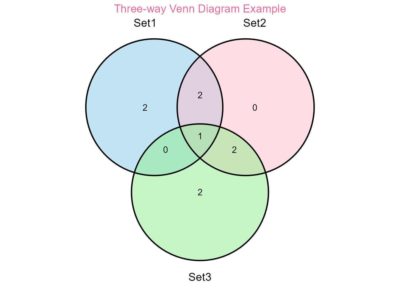
Venn diagram example
Bar Plots
# Sample data
sample_data <- data.frame(
  Category = c("Type A", "Type B", "Type C"),
  Count = c(25, 18, 12),
  Group = c("High", "High", "Medium")
)

# Create bar plot with custom colors
vivid_colors <- get_palette("qual_vivid", type = "qualitative")
bar_plot <- plot_bar(data = sample_data,
                     x = "Category",
                     y = "Count",
                     fill = "Group") +
  ggplot2::scale_fill_manual(values = vivid_colors) +
  ggplot2::labs(title = "Sample Distribution by Category",
                x = "Sample Type",
                y = "Count")
print(bar_plot)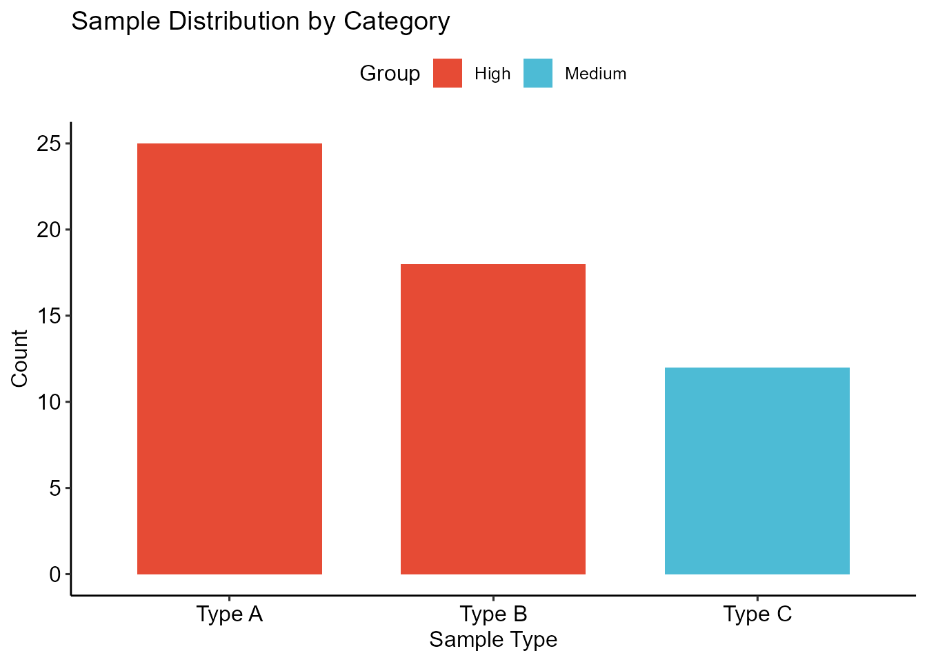
Professional bar plot
🧬 Bioinformatics Utilities
Gene ID Conversion
# Convert gene symbols to Ensembl IDs
gene_symbols <- c("TP53", "BRCA1", "EGFR")
ensembl_ids <- convert_gene_id(
  ids = gene_symbols,
  from = "SYMBOL",
  to = "ENSEMBL",
  species = "human"
)
print(ensembl_ids)🔄 Data Processing and Void Handling
Working with Void Values
# Create sample vector with void values
messy_vector <- c("A", "", "C", NA, "E")

print("Original vector:")
#> [1] "Original vector:"
print(messy_vector)
#> [1] "A" ""  "C" NA  "E"

# Check for void values
cat("\nAny void values:", any_void(messy_vector), "\n")
#>
#> Any void values: TRUE

# Replace void values
clean_vector <- replace_void(messy_vector, value = "MISSING")
print("After replacing voids:")
#> [1] "After replacing voids:"
print(clean_vector)
#> [1] "A"       "MISSING" "C"       "MISSING" "E"
Data Transformation
# Convert data frame to grouped list by cylinder count
grouped_data <- df2list(
  data = mtcars[1:10, ],
  key_col = "cyl",
  value_col = "mpg"
)

print("Cars grouped by cylinder, showing MPG values:")
#> [1] "Cars grouped by cylinder, showing MPG values:"
str(grouped_data)
#> List of 3
#>  $ 4: num [1:3] 22.8 24.4 22.8
#>  $ 6: num [1:5] 21 21 21.4 18.1 19.2
#> $ 8: num [1:2] 18.7 14.3💾 File Operations
Flexible File Reading
# Read various file formats flexibly
data1 <- read_table_flex("data.csv")
data2 <- read_excel_flex("data.xlsx", sheet = 1)

# Get file information
file_info("data.csv")

# Display directory tree
file_tree(".")
🛠️ Development Tools
Timing and Execution
# Time execution of code
result <- with_timer(function() {
  Sys.sleep(0.01)  # Quick simulation
  sum(1:1000)
}, name = "Sum calculation")

print(result)
#> function (...)
#> {
#>     cli::cli_alert_info("{name} started at {format(Sys.time(), '%Y-%m-%d %H:%M:%S')}")
#>     tictoc::tic()
#>     result <- fn(...)
#>     timing <- tictoc::toc(quiet = TRUE)
#>     elapsed <- as.numeric(timing$toc - timing$tic, units = "secs")
#>     cli::cli_alert_success("{name} completed in {sprintf('%.3f', elapsed)} seconds")
#>     invisible(result)
#> }
#> <bytecode: 0x55dc83728c80>
#> <environment: 0x55dc8372bd20>
Safe Execution
# Execute code safely
safe_result <- safe_execute({
  x <- 1:10
  mean(x)
})

print(safe_result)
#> [1] 5.5
📈 Summary
The evanverse package provides a comprehensive toolkit for:
- Package Management: Multi-source installation and management
- Data Visualization: Publication-ready plots with sensible defaults
- Color Management: Professional palette system for consistent styling
- File Operations: Robust I/O with enhanced error handling
- Bioinformatics: Specialized tools for genomic data processing
- Data Processing: Advanced transformation and void value handling
- Custom Operators: Expressive syntax extensions for R
- Development Tools: Productivity enhancing utilities
With 55+ functions across 8 major categories, evanverse streamlines your data analysis workflow while maintaining flexibility and reliability.
🔗 Next Steps
- Explore the Color Palettes guide for advanced palette management
- Check out Bioinformatics Workflows for domain-specific applications
- Visit the Function Reference for detailed documentation
For more information, visit the evanverse website or the GitHub repository.