Bioinformatics Workflows with evanverse
Source:vignettes/bioinformatics-workflows.Rmd
bioinformatics-workflows.Rmd🧬 Bioinformatics Workflows with evanverse
The evanverse package provides specialized tools for
common bioinformatics workflows, including gene ID conversion, gene set
analysis, pathway enrichment visualization, and biological data download
utilities. This comprehensive guide demonstrates practical applications
in genomics and systems biology.
🎯 Overview of Bioinformatics Functions
Core Bioinformatics Tools
| Function | Purpose | Common Use Cases |
|---|---|---|
convert_gene_id() |
Gene identifier conversion | Symbol ↔︎ Ensembl, Entrez ↔︎ Symbol |
download_gene_ref() |
Reference genome downloads | Annotation files, gene models |
gmt2df() |
GMT file to data frame | Pathway analysis, gene set processing |
gmt2list() |
GMT file to named list | Enrichment analysis, functional annotation |
download_geo_data() |
GEO data retrieval | Public dataset analysis |
plot_venn() |
Venn diagram analysis | Gene set overlaps, differential expression |
🔄 Gene Identifier Conversion
Basic Gene ID Conversion
Gene identifier conversion is fundamental in bioinformatics for integrating datasets from different sources.
# Example gene symbols commonly used in cancer research
cancer_genes <- c("BRCA1", "BRCA2", "TP53", "EGFR", "MYC", "RAS", "PIK3CA", "AKT1")

# Convert gene symbols to Ensembl IDs
ensembl_ids <- convert_gene_id(
  genes = cancer_genes,
  from = "symbol",
  to = "ensembl",
  species = "human"
)

# Display conversion results
conversion_table <- data.frame(
  Gene_Symbol = cancer_genes,
  Ensembl_ID = ensembl_ids
)

print(conversion_table)
# Mock example for demonstration (since biomaRt requires internet)
cancer_genes <- c("BRCA1", "BRCA2", "TP53", "EGFR", "MYC", "KRAS", "PIK3CA", "AKT1")

# Simulated conversion results
mock_conversion <- data.frame(
  Gene_Symbol = cancer_genes,
  Ensembl_ID = c(
    "ENSG00000012048", "ENSG00000139618", "ENSG00000141510",
    "ENSG00000146648", "ENSG00000136997", "ENSG00000133703",
    "ENSG00000171608", "ENSG00000142208"
  ),
  Entrez_ID = c(672, 675, 7157, 1956, 4609, 3845, 5290, 207),
  stringsAsFactors = FALSE
)

cat("🧬 Gene ID Conversion Example\n")
#> 🧬 Gene ID Conversion Example
cat("=============================\n")
#> =============================
print(mock_conversion)
#>   Gene_Symbol      Ensembl_ID Entrez_ID
#> 1       BRCA1 ENSG00000012048       672
#> 2       BRCA2 ENSG00000139618       675
#> 3        TP53 ENSG00000141510      7157
#> 4        EGFR ENSG00000146648      1956
#> 5         MYC ENSG00000136997      4609
#> 6        KRAS ENSG00000133703      3845
#> 7      PIK3CA ENSG00000171608      5290
#> 8        AKT1 ENSG00000142208       207

cat("\n📊 Conversion Summary:\n")
#>
#> 📊 Conversion Summary:
cat("  • Input genes:", length(cancer_genes), "\n")
#>   • Input genes: 8
cat("  • Successful conversions:", nrow(mock_conversion), "\n")
#>   • Successful conversions: 8
cat("  • Success rate:", round(100 * nrow(mock_conversion) / length(cancer_genes), 1), "%\n")
#>   • Success rate: 100 %
Advanced Conversion Workflows
# Simulate a real-world scenario with mixed identifier types
mixed_identifiers <- c(
  "BRCA1", "ENSG00000139618", "7157", "EGFR",
  "ENSG00000136997", "3845", "PIK3CA", "207"
)

# Function to detect identifier type
detect_id_type <- function(ids) {
  sapply(ids, function(id) {
    if (grepl("^ENSG", id)) return("ensembl")
    if (grepl("^[0-9]+$", id)) return("entrez")
    return("symbol")
  })
}

id_types <- detect_id_type(mixed_identifiers)
cat("🔍 Identifier Type Detection:\n")
#> 🔍 Identifier Type Detection:
print(data.frame(
  Identifier = mixed_identifiers,
  Detected_Type = id_types
))
#>                      Identifier Detected_Type
#> BRCA1                     BRCA1        symbol
#> ENSG00000139618 ENSG00000139618       ensembl
#> 7157                       7157        entrez
#> EGFR                       EGFR        symbol
#> ENSG00000136997 ENSG00000136997       ensembl
#> 3845                       3845        entrez
#> PIK3CA                   PIK3CA        symbol
#> 207                         207        entrez

# Group by identifier type for batch conversion
id_groups <- split(mixed_identifiers, id_types)
cat("\n📦 Grouped Identifiers for Conversion:\n")
#>
#> 📦 Grouped Identifiers for Conversion:
str(id_groups)
#> List of 3
#>  $ ensembl: chr [1:2] "ENSG00000139618" "ENSG00000136997"
#>  $ entrez : chr [1:3] "7157" "3845" "207"
#>  $ symbol : chr [1:3] "BRCA1" "EGFR" "PIK3CA"
📊 Gene Set Analysis with GMT Files
Processing GMT Files
GMT (Gene Matrix Transposed) files are standard formats for gene set collections used in pathway analysis.
# Example: Process a pathway GMT file
# pathway_df <- gmt2df("path/to/c2.cp.kegg.v7.4.symbols.gmt")
# pathway_list <- gmt2list("path/to/c2.cp.kegg.v7.4.symbols.gmt")

# Display structure
# head(pathway_df, 10)
# length(pathway_list)
# Create mock GMT data to demonstrate structure
mock_pathways <- list(
  "KEGG_GLYCOLYSIS_GLUCONEOGENESIS" = c(
    "HK1", "HK2", "GPI", "PFKL", "ALDOA", "TPI1", "GAPDH",
    "PGK1", "PGAM1", "ENO1", "PKM", "LDHA", "PDK1"
  ),
  "KEGG_CITRATE_CYCLE" = c(
    "CS", "ACO1", "IDH1", "OGDH", "SUCLA2", "SDHA",
    "FH", "MDH1", "PCK1", "PDK1", "DLAT"
  ),
  "KEGG_FATTY_ACID_SYNTHESIS" = c(
    "ACACA", "FASN", "ACLY", "ACC2", "ELOVL6", "SCD",
    "FADS1", "FADS2", "ACSL1", "GPAM"
  ),
  "KEGG_DNA_REPAIR" = c(
    "BRCA1", "BRCA2", "TP53", "ATM", "CHEK1", "CHEK2",
    "RAD51", "XRCC1", "PARP1", "MSH2", "MLH1"
  )
)

# Convert list to data frame format (simulating gmt2df output)
mock_gmt_df <- do.call(rbind, lapply(names(mock_pathways), function(pathway) {
  data.frame(
    pathway = pathway,
    gene = mock_pathways[[pathway]],
    stringsAsFactors = FALSE
  )
}))

cat("📋 GMT File Processing Results\n")
#> 📋 GMT File Processing Results
cat("==============================\n")
#> ==============================
cat("Number of pathways:", length(mock_pathways), "\n")
#> Number of pathways: 4
cat("Total gene-pathway associations:", nrow(mock_gmt_df), "\n")
#> Total gene-pathway associations: 45
cat("Average genes per pathway:", round(mean(lengths(mock_pathways)), 1), "\n\n")
#> Average genes per pathway: 11.2

cat("Sample pathway data frame:\n")
#> Sample pathway data frame:
print(head(mock_gmt_df, 12))
#>                            pathway  gene
#> 1  KEGG_GLYCOLYSIS_GLUCONEOGENESIS   HK1
#> 2  KEGG_GLYCOLYSIS_GLUCONEOGENESIS   HK2
#> 3  KEGG_GLYCOLYSIS_GLUCONEOGENESIS   GPI
#> 4  KEGG_GLYCOLYSIS_GLUCONEOGENESIS  PFKL
#> 5  KEGG_GLYCOLYSIS_GLUCONEOGENESIS ALDOA
#> 6  KEGG_GLYCOLYSIS_GLUCONEOGENESIS  TPI1
#> 7  KEGG_GLYCOLYSIS_GLUCONEOGENESIS GAPDH
#> 8  KEGG_GLYCOLYSIS_GLUCONEOGENESIS  PGK1
#> 9  KEGG_GLYCOLYSIS_GLUCONEOGENESIS PGAM1
#> 10 KEGG_GLYCOLYSIS_GLUCONEOGENESIS  ENO1
#> 11 KEGG_GLYCOLYSIS_GLUCONEOGENESIS   PKM
#> 12 KEGG_GLYCOLYSIS_GLUCONEOGENESIS  LDHA

# Pathway size distribution
pathway_sizes <- lengths(mock_pathways)
cat("\n📊 Pathway Size Distribution:\n")
#>
#> 📊 Pathway Size Distribution:
print(data.frame(
  Pathway = names(pathway_sizes),
  Gene_Count = pathway_sizes
))
#>                                                         Pathway Gene_Count
#> KEGG_GLYCOLYSIS_GLUCONEOGENESIS KEGG_GLYCOLYSIS_GLUCONEOGENESIS         13
#> KEGG_CITRATE_CYCLE                           KEGG_CITRATE_CYCLE         11
#> KEGG_FATTY_ACID_SYNTHESIS             KEGG_FATTY_ACID_SYNTHESIS         10
#> KEGG_DNA_REPAIR                                 KEGG_DNA_REPAIR         11
Gene Set Overlap Analysis
# Analyze overlaps between pathways
pathway_genes <- mock_pathways[1:3]  # Use first 3 pathways for Venn diagram

# Create Venn diagram for pathway overlaps
venn_plot <- plot_venn(
  set1 = pathway_genes[[1]],
  set2 = pathway_genes[[2]],
  set3 = pathway_genes[[3]],
  category.names = names(pathway_genes),
  fill = get_palette("qual_vivid", type = "qualitative", n = 3),
  title = "Metabolic Pathway Gene Overlaps"
)
#> ✔ Loaded palette "qual_vivid" ("qualitative"), 9 colors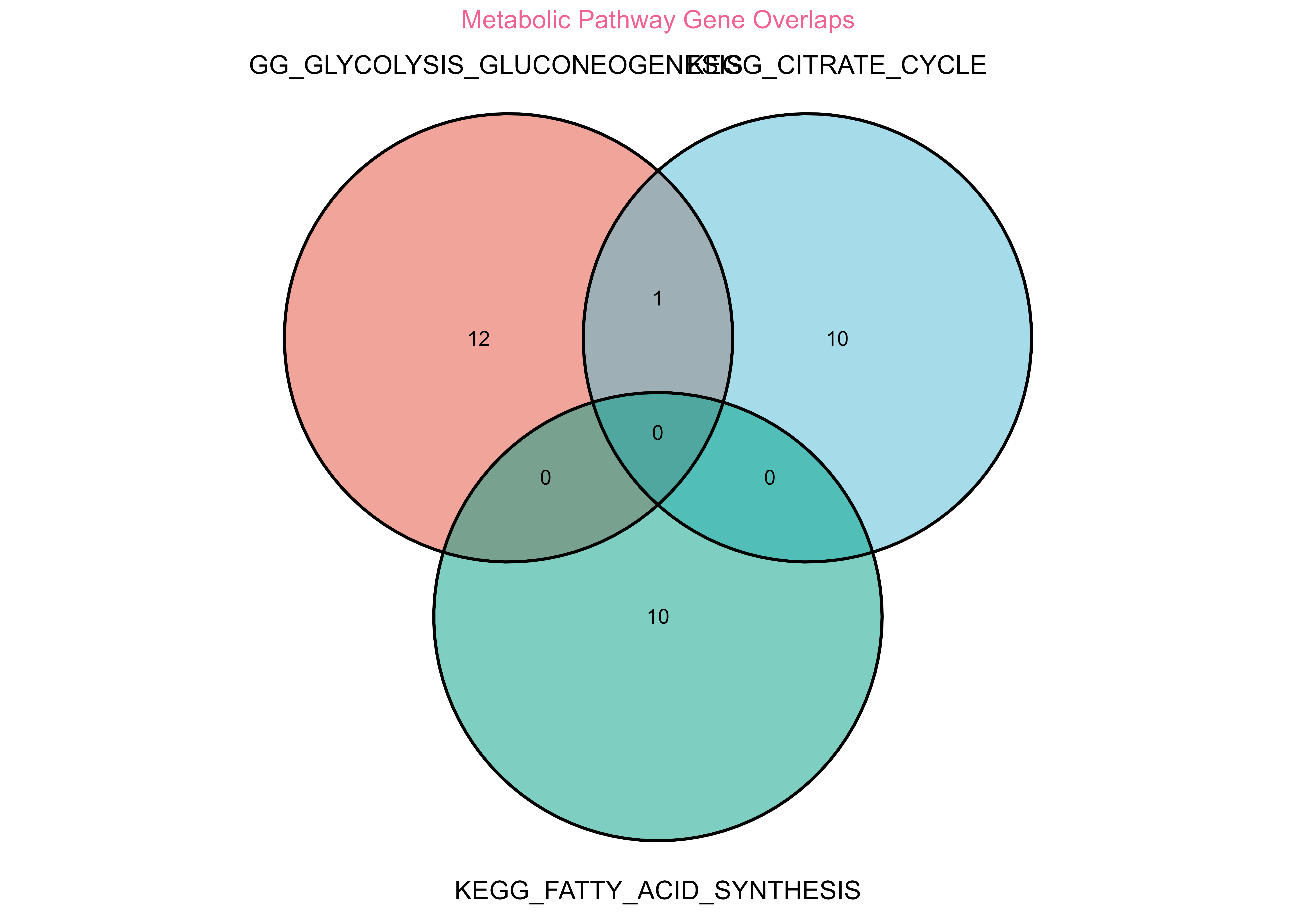
Gene set overlap analysis showing relationships between biological pathways
print(venn_plot)
Gene set overlap analysis showing relationships between biological pathways
# Calculate detailed overlap statistics
all_genes <- unique(unlist(pathway_genes))
cat("\n🔍 Detailed Overlap Analysis:\n")
#>
#> 🔍 Detailed Overlap Analysis:
cat("===============================\n")
#> ===============================
cat("Total unique genes across pathways:", length(all_genes), "\n")
#> Total unique genes across pathways: 33

# Pairwise overlaps
pathway_names <- names(pathway_genes)
for (i in 1:(length(pathway_names) - 1)) {
  for (j in (i + 1):length(pathway_names)) {
    overlap <- length(intersect(pathway_genes[[i]], pathway_genes[[j]]))
    cat(sprintf("%s ∩ %s: %d genes\n",
                gsub("KEGG_", "", pathway_names[i]),
                gsub("KEGG_", "", pathway_names[j]),
                overlap))
  }
}
#> GLYCOLYSIS_GLUCONEOGENESIS ∩ CITRATE_CYCLE: 1 genes
#> GLYCOLYSIS_GLUCONEOGENESIS ∩ FATTY_ACID_SYNTHESIS: 0 genes
#> CITRATE_CYCLE ∩ FATTY_ACID_SYNTHESIS: 0 genes
🎯 Differential Expression Analysis Workflow
Simulated RNA-seq Analysis
# Simulate RNA-seq differential expression results
set.seed(123)
n_genes <- 2000

# Simulate log fold changes and p-values
gene_results <- data.frame(
  Gene = paste0("Gene_", 1:n_genes),
  LogFC = rnorm(n_genes, mean = 0, sd = 1.2),
  PValue = rbeta(n_genes, shape1 = 1, shape2 = 10),
  stringsAsFactors = FALSE
)

# Add some significant genes
significant_indices <- sample(1:n_genes, 200)
gene_results$LogFC[significant_indices] <- gene_results$LogFC[significant_indices] +
  sample(c(-2, 2), 200, replace = TRUE)
gene_results$PValue[significant_indices] <- gene_results$PValue[significant_indices] * 0.01

# Calculate adjusted p-values
gene_results$FDR <- p.adjust(gene_results$PValue, method = "BH")

# Classify genes
gene_results$Regulation <- "Not Significant"
gene_results$Regulation[gene_results$FDR < 0.05 & gene_results$LogFC > 1] <- "Up-regulated"
gene_results$Regulation[gene_results$FDR < 0.05 & gene_results$LogFC < -1] <- "Down-regulated"

# Create volcano plot
volcano_colors <- c(
  "Up-regulated" = get_palette("qual_vivid", type = "qualitative", n = 3)[1],
  "Down-regulated" = get_palette("qual_vivid", type = "qualitative", n = 3)[2],
  "Not Significant" = "#CCCCCC"
)
#> ✔ Loaded palette "qual_vivid" ("qualitative"), 9 colors
#> ✔ Loaded palette "qual_vivid" ("qualitative"), 9 colors

p1 <- ggplot(gene_results, aes(x = LogFC, y = -log10(FDR), color = Regulation)) +
  geom_point(alpha = 0.6, size = 1.2) +
  scale_color_manual(values = volcano_colors) +
  geom_vline(xintercept = c(-1, 1), linetype = "dashed", color = "#666666") +
  geom_hline(yintercept = -log10(0.05), linetype = "dashed", color = "#666666") +
  labs(
    title = "Differential Gene Expression Analysis",
    subtitle = "Volcano plot showing treatment vs. control comparison",
    x = "Log₂ Fold Change",
    y = "-log₁₀(FDR-adjusted p-value)",
    color = "Regulation"
  ) +
  theme_minimal() +
  theme(
    plot.title = element_text(size = 14, face = "bold", color = "#0D47A1"),
    plot.subtitle = element_text(size = 11, color = "#666666"),
    legend.position = "bottom"
  )

print(p1)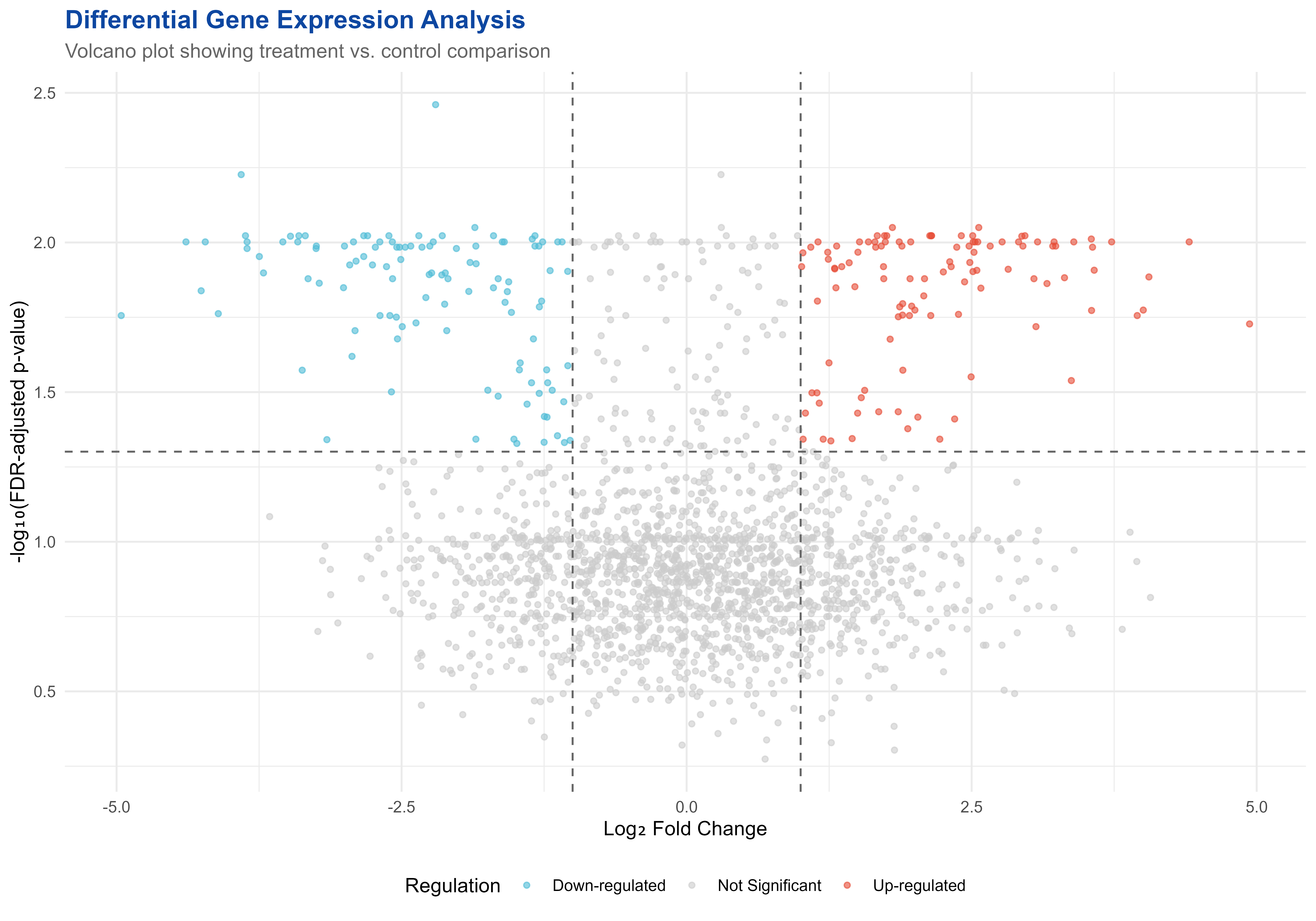
Differential expression analysis visualization with volcano plot
# Summary statistics
regulation_summary <- table(gene_results$Regulation)
cat("\n📊 Differential Expression Summary:\n")
#>
#> 📊 Differential Expression Summary:
cat("===================================\n")
#> ===================================
print(regulation_summary)
#>
#>  Down-regulated Not Significant    Up-regulated
#>             113            1777             110

cat("\nTop 10 up-regulated genes (by fold change):\n")
#>
#> Top 10 up-regulated genes (by fold change):
top_up <- gene_results[gene_results$Regulation == "Up-regulated", ] %>%
  arrange(desc(LogFC)) %>%
  head(10)
print(top_up[, c("Gene", "LogFC", "FDR")])
#>         Gene    LogFC         FDR
#> 1  Gene_1911 4.937598 0.018718628
#> 2   Gene_948 4.408017 0.009956437
#> 3   Gene_477 4.054766 0.013037421
#> 4   Gene_343 4.005266 0.016821175
#> 5   Gene_489 3.952257 0.017546948
#> 6  Gene_1189 3.727714 0.009956437
#> 7   Gene_202 3.574896 0.012378355
#> 8   Gene_264 3.560238 0.010369230
#> 9  Gene_1926 3.551683 0.016873989
#> 10 Gene_1255 3.549588 0.009735872
Pathway Enrichment Analysis
# Simulate pathway enrichment analysis results
enrichment_results <- data.frame(
  Pathway = c(
    "Cell Cycle", "Apoptosis", "DNA Repair", "Inflammation",
    "Metabolism", "Signaling", "Transport", "Development"
  ),
  GeneRatio = c(0.15, 0.22, 0.18, 0.31, 0.09, 0.25, 0.12, 0.08),
  FDR = c(0.001, 0.003, 0.008, 0.0001, 0.045, 0.002, 0.021, 0.089),
  GeneCount = c(23, 34, 28, 48, 14, 39, 18, 12),
  stringsAsFactors = FALSE
)

# Calculate enrichment score
enrichment_results$EnrichmentScore <- -log10(enrichment_results$FDR)

# Create enrichment plot
p2 <- ggplot(enrichment_results, aes(x = GeneRatio, y = reorder(Pathway, EnrichmentScore))) +
  geom_point(aes(color = EnrichmentScore, size = GeneCount), alpha = 0.8) +
  scale_color_gradientn(
    colors = get_palette("seq_blush", type = "sequential", n = 4),
    name = "-log₁₀(FDR)"
  ) +
  scale_size_continuous(name = "Gene Count", range = c(3, 12)) +
  geom_vline(xintercept = 0.1, linetype = "dashed", color = "#666666", alpha = 0.7) +
  labs(
    title = "Pathway Enrichment Analysis",
    subtitle = "Biological processes enriched in differentially expressed genes",
    x = "Gene Ratio (enriched genes / pathway total)",
    y = "Biological Pathway"
  ) +
  theme_minimal() +
  theme(
    plot.title = element_text(size = 14, face = "bold", color = "#0D47A1"),
    plot.subtitle = element_text(size = 11, color = "#666666"),
    panel.grid.major.y = element_blank(),
    legend.position = "right"
  )
#> ✔ Loaded palette "seq_blush" ("sequential"), 4 colors

print(p2)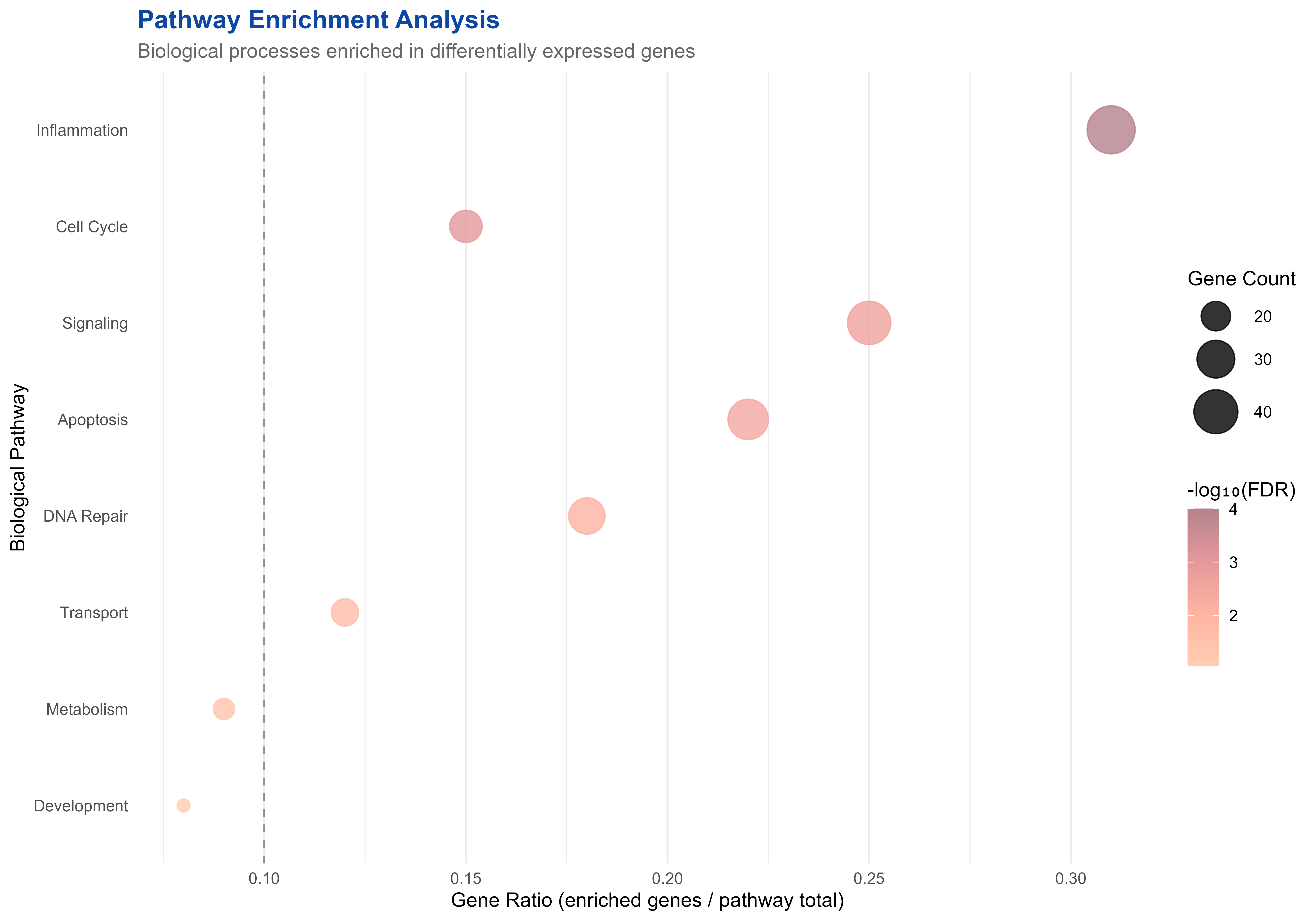
Pathway enrichment analysis showing biological processes affected by treatment
cat("\n🎯 Pathway Enrichment Summary:\n")
#>
#> 🎯 Pathway Enrichment Summary:
cat("==============================\n")
#> ==============================
significant_pathways <- enrichment_results[enrichment_results$FDR < 0.05, ]
cat("Significant pathways (FDR < 0.05):", nrow(significant_pathways), "\n")
#> Significant pathways (FDR < 0.05): 7
cat("Most enriched pathway:", significant_pathways$Pathway[which.max(significant_pathways$EnrichmentScore)], "\n")
#> Most enriched pathway: Inflammation
cat("Total genes in significant pathways:", sum(significant_pathways$GeneCount), "\n")
#> Total genes in significant pathways: 204
🌐 Multi-omics Integration
Combining Genomics and Transcriptomics
# Simulate multi-omics data integration
set.seed(456)
selected_genes <- c("BRCA1", "TP53", "EGFR", "MYC", "KRAS", "PIK3CA", "AKT1", "PTEN")

# Create integrated omics data
omics_data <- data.frame(
  Gene = rep(selected_genes, each = 3),
  DataType = rep(c("Mutation", "CNV", "Expression"), length(selected_genes)),
  Value = c(
    # Mutation frequencies (0-1)
    c(0.12, 0.34, 0.08, 0.15, 0.22, 0.09, 0.06, 0.18),
    # Copy number variations (-2 to 2)
    c(-0.5, -1.2, 1.8, 0.3, 0.8, -0.8, 1.1, -1.5),
    # Expression fold changes (-3 to 3)
    c(-1.5, -2.8, 2.1, 1.8, -1.2, 2.3, -0.8, -2.1)
  ),
  Patient_Group = rep(c("Group_A", "Group_B", "Group_C"), length(selected_genes))
)

# Normalize values for visualization
omics_data$Normalized_Value <- ave(omics_data$Value, omics_data$DataType,
                                   FUN = function(x) scale(x)[,1])

# Create heatmap
p3 <- ggplot(omics_data, aes(x = DataType, y = Gene, fill = Normalized_Value)) +
  geom_tile(color = "white", size = 0.5) +
  scale_fill_gradientn(
    colors = get_palette("div_contrast", type = "diverging"),
    name = "Z-score",
    limits = c(-2, 2),
    breaks = c(-2, -1, 0, 1, 2)
  ) +
  labs(
    title = "Multi-omics Cancer Gene Analysis",
    subtitle = "Integrated view of mutations, copy number, and expression",
    x = "Data Type",
    y = "Cancer-related Genes"
  ) +
  theme_minimal() +
  theme(
    plot.title = element_text(size = 14, face = "bold", color = "#0D47A1"),
    plot.subtitle = element_text(size = 11, color = "#666666"),
    panel.grid = element_blank(),
    axis.text.x = element_text(angle = 45, hjust = 1)
  )
#> Warning: Using `size` aesthetic for lines was deprecated in ggplot2 3.4.0.
#> ℹ Please use `linewidth` instead.
#> This warning is displayed once per session.
#> Call `lifecycle::last_lifecycle_warnings()` to see where this warning was
#> generated.
#> ✔ Loaded palette "div_contrast" ("diverging"), 2 colors

print(p3)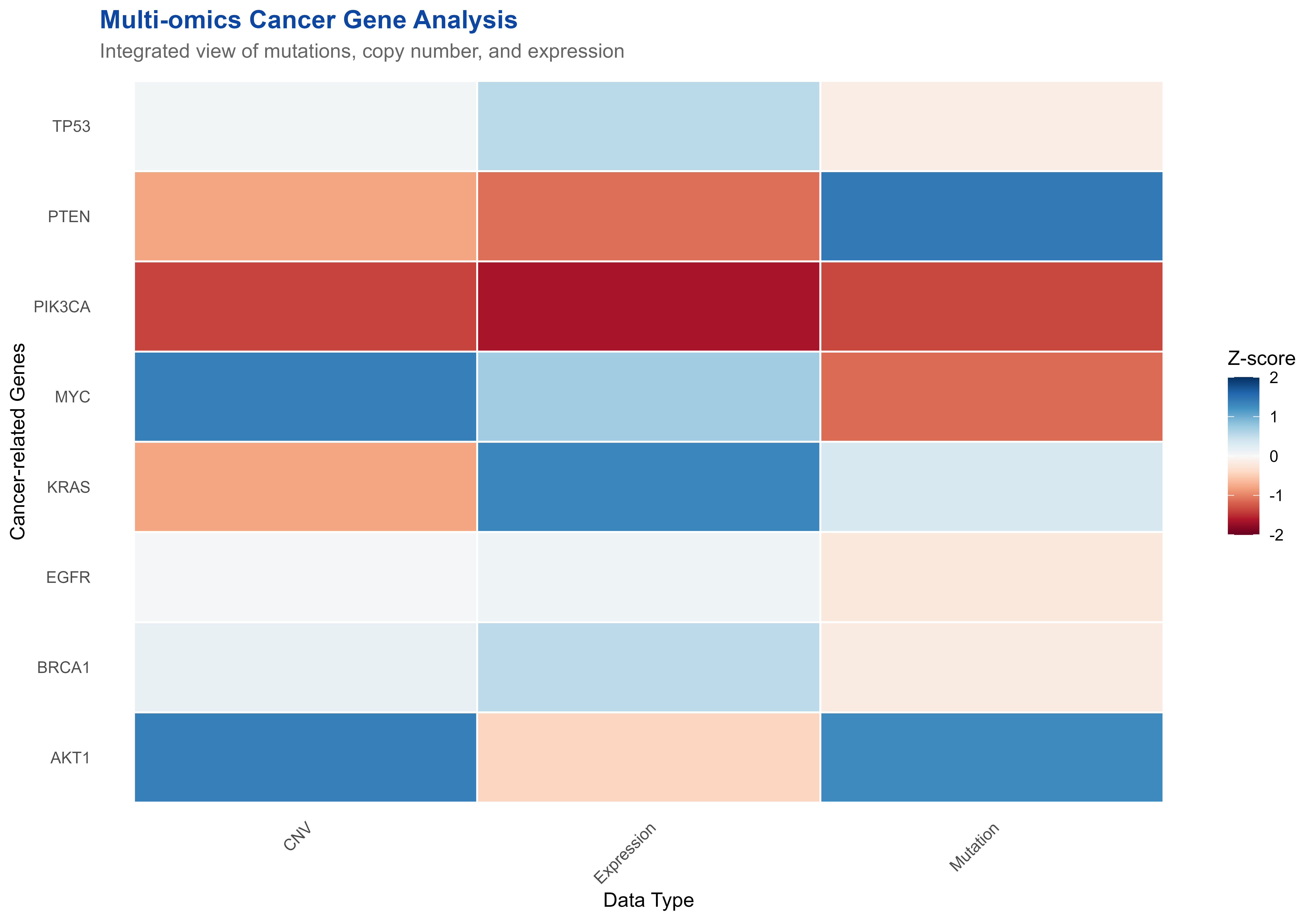
Multi-omics data integration showing genomic variants and expression changes
# Summary by data type
cat("\n🧬 Multi-omics Data Summary:\n")
#>
#> 🧬 Multi-omics Data Summary:
cat("============================\n")
#> ============================
summary_stats <- omics_data %>%
  group_by(DataType) %>%
  summarise(
    Mean_Value = round(mean(Value), 3),
    SD_Value = round(sd(Value), 3),
    Min_Value = round(min(Value), 3),
    Max_Value = round(max(Value), 3),
    .groups = 'drop'
  )
print(summary_stats)
#> # A tibble: 3 × 5
#>   DataType   Mean_Value SD_Value Min_Value Max_Value
#>   <chr>           <dbl>    <dbl>     <dbl>     <dbl>
#> 1 CNV             0.155     1.20      -1.5       1.8
#> 2 Expression     -0.629     1.31      -2.8       1.1
#> 3 Mutation        0.354     1.37      -1.5       2.3
🔬 Clinical Data Integration
Biomarker Discovery Pipeline
# Simulate clinical biomarker data
set.seed(789)
n_patients <- 120
n_biomarkers <- 20

# Generate patient clinical data
clinical_data <- data.frame(
  Patient_ID = paste0("P", 1:n_patients),
  Subtype = sample(c("Luminal_A", "Luminal_B", "HER2+", "TNBC"), n_patients,
                   replace = TRUE, prob = c(0.4, 0.2, 0.15, 0.25)),
  Stage = sample(c("I", "II", "III", "IV"), n_patients,
                 replace = TRUE, prob = c(0.3, 0.35, 0.25, 0.1)),
  Age = round(rnorm(n_patients, 55, 12)),
  Survival_Months = round(rexp(n_patients, rate = 0.02)),
  stringsAsFactors = FALSE
)

# Generate biomarker expression data
biomarker_genes <- paste0("Biomarker_", 1:n_biomarkers)
expression_data <- matrix(rnorm(n_patients * n_biomarkers, mean = 5, sd = 2),
                         nrow = n_patients, ncol = n_biomarkers)
colnames(expression_data) <- biomarker_genes
rownames(expression_data) <- clinical_data$Patient_ID

# Add subtype-specific expression patterns
luminal_a_patients <- clinical_data$Patient_ID[clinical_data$Subtype == "Luminal_A"]
her2_patients <- clinical_data$Patient_ID[clinical_data$Subtype == "HER2+"]
tnbc_patients <- clinical_data$Patient_ID[clinical_data$Subtype == "TNBC"]

# Simulate subtype-specific biomarkers
expression_data[luminal_a_patients, "Biomarker_1"] <-
  expression_data[luminal_a_patients, "Biomarker_1"] + 3

expression_data[her2_patients, "Biomarker_5"] <-
  expression_data[her2_patients, "Biomarker_5"] + 4

expression_data[tnbc_patients, "Biomarker_12"] <-
  expression_data[tnbc_patients, "Biomarker_12"] + 2.5

# Convert to long format for visualization
expression_long <- as.data.frame(expression_data) %>%
  mutate(Patient_ID = rownames(.)) %>%
  gather(Biomarker, Expression, -Patient_ID) %>%
  left_join(clinical_data, by = "Patient_ID")

# Select top biomarkers for visualization
top_biomarkers <- c("Biomarker_1", "Biomarker_5", "Biomarker_12", "Biomarker_8")
plot_data <- expression_long %>%
  filter(Biomarker %in% top_biomarkers)

# Create biomarker expression plot
p5 <- ggplot(plot_data, aes(x = Subtype, y = Expression, fill = Subtype)) +
  geom_boxplot(alpha = 0.7, outlier.alpha = 0.5) +
  geom_jitter(alpha = 0.3, width = 0.2, size = 0.8) +
  scale_fill_manual(
    values = get_palette("qual_vivid", type = "qualitative", n = 4)
  ) +
  facet_wrap(~Biomarker, scales = "free_y", ncol = 2) +
  labs(
    title = "Biomarker Expression Across Cancer Subtypes",
    subtitle = "Potential subtype-specific biomarkers for precision medicine",
    x = "Cancer Subtype",
    y = "Expression Level (log2 normalized)",
    fill = "Subtype"
  ) +
  theme_minimal() +
  theme(
    plot.title = element_text(size = 14, face = "bold", color = "#0D47A1"),
    plot.subtitle = element_text(size = 11, color = "#666666"),
    axis.text.x = element_text(angle = 45, hjust = 1),
    legend.position = "bottom",
    strip.background = element_rect(fill = "#E3F2FD", color = NA)
  )
#> ✔ Loaded palette "qual_vivid" ("qualitative"), 9 colors

print(p5)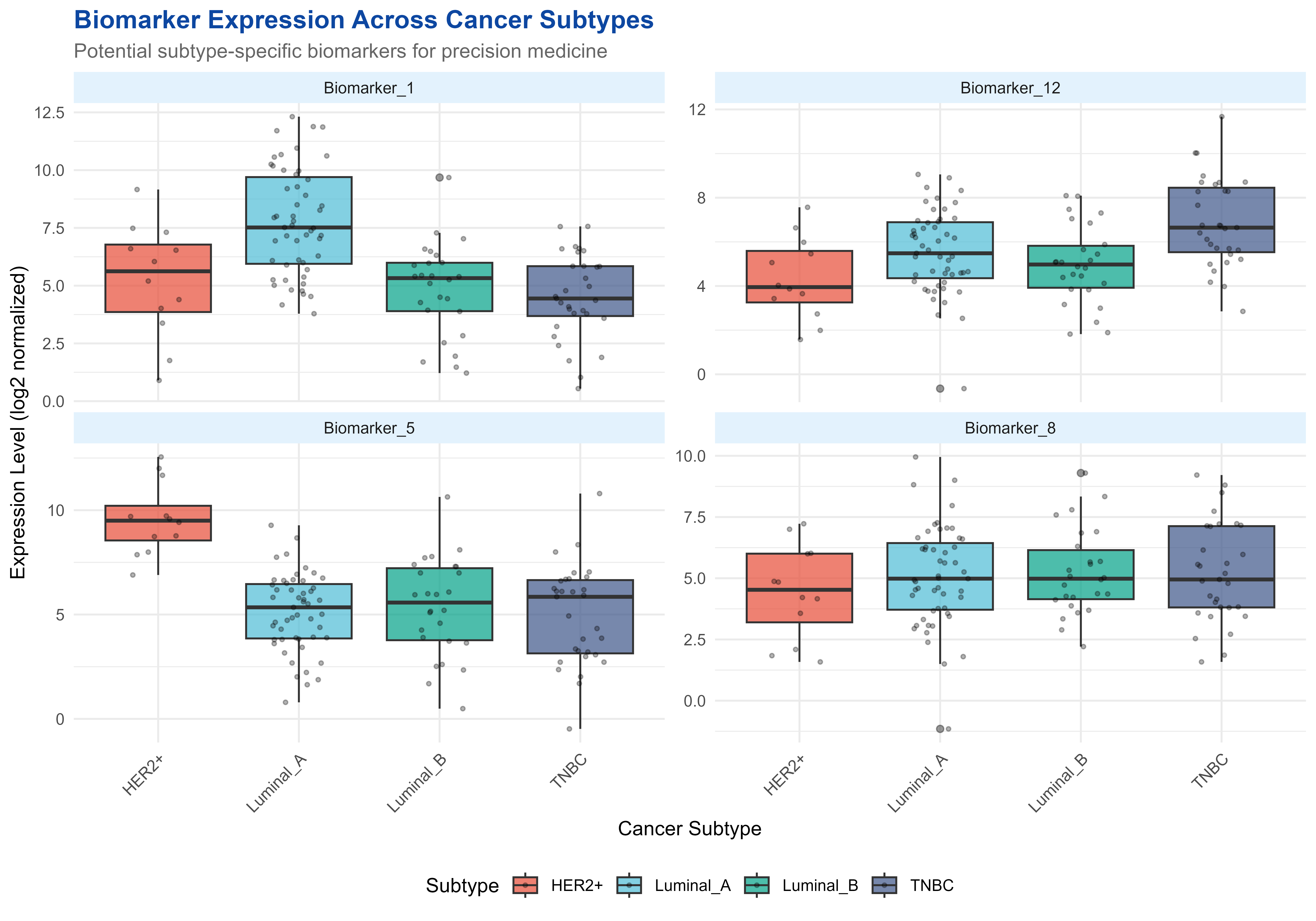
Biomarker discovery showing gene expression patterns across clinical subtypes
# Statistical summary
cat("\n📊 Biomarker Analysis Summary:\n")
#>
#> 📊 Biomarker Analysis Summary:
cat("==============================\n")
#> ==============================
subtype_counts <- table(clinical_data$Subtype)
print(subtype_counts)
#>
#>     HER2+ Luminal_A Luminal_B      TNBC
#>        12        51        26        31

cat("\nMean expression by subtype for key biomarkers:\n")
#>
#> Mean expression by subtype for key biomarkers:
biomarker_summary <- plot_data %>%
  group_by(Biomarker, Subtype) %>%
  summarise(
    Mean_Expression = round(mean(Expression), 2),
    SD = round(sd(Expression), 2),
    .groups = 'drop'
  ) %>%
  arrange(Biomarker, desc(Mean_Expression))

print(biomarker_summary)
#> # A tibble: 16 × 4
#>    Biomarker    Subtype   Mean_Expression    SD
#>    <chr>        <chr>               <dbl> <dbl>
#>  1 Biomarker_1  Luminal_A            7.76  2.29
#>  2 Biomarker_1  HER2+                5.23  2.44
#>  3 Biomarker_1  Luminal_B            4.84  2.02
#>  4 Biomarker_1  TNBC                 4.54  1.84
#>  5 Biomarker_12 TNBC                 6.88  2.01
#>  6 Biomarker_12 Luminal_A            5.55  1.87
#>  7 Biomarker_12 Luminal_B            4.97  1.77
#>  8 Biomarker_12 HER2+                4.33  1.85
#>  9 Biomarker_5  HER2+                9.58  1.74
#> 10 Biomarker_5  Luminal_B            5.36  2.34
#> 11 Biomarker_5  Luminal_A            5.11  1.85
#> 12 Biomarker_5  TNBC                 4.98  2.37
#> 13 Biomarker_8  Luminal_B            5.23  1.74
#> 14 Biomarker_8  TNBC                 5.22  2.03
#> 15 Biomarker_8  Luminal_A            5.08  2.05
#> 16 Biomarker_8  HER2+                4.45  1.93
🛠️ Data Download and Management
Public Dataset Retrieval
# Example of downloading reference data
# Note: These functions require internet connection and may take time

# Download gene reference annotation
gene_ref <- download_gene_ref(
  species = "human",
  build = "hg38",
  feature_type = "gene"
)

# Download GEO dataset
geo_data <- download_geo_data(
  geo_id = "GSE123456",
  destdir = "data/geo_downloads"
)

# Download pathway databases
pathway_url <- "https://data.broadinstitute.org/gsea-msigdb/msigdb/release/7.4/c2.cp.kegg.v7.4.symbols.gmt"
download_url(
  url = pathway_url,
  dest = "data/pathways/kegg_pathways.gmt"
)
# Demonstrate file organization for bioinformatics projects
cat("📁 Recommended Project Structure for Bioinformatics:\n")
#> 📁 Recommended Project Structure for Bioinformatics:
cat("==================================================\n")
#> ==================================================
cat("project/\n")
#> project/
cat("├── data/\n")
#> ├── data/
cat("│   ├── raw/                 # Original data files\n")
#> │   ├── raw/                 # Original data files
cat("│   ├── processed/           # Cleaned/normalized data\n")
#> │   ├── processed/           # Cleaned/normalized data
cat("│   ├── reference/           # Genome annotations, databases\n")
#> │   ├── reference/           # Genome annotations, databases
cat("│   └── results/             # Analysis outputs\n")
#> │   └── results/             # Analysis outputs
cat("├── scripts/\n")
#> ├── scripts/
cat("│   ├── preprocessing/       # Data cleaning scripts\n")
#> │   ├── preprocessing/       # Data cleaning scripts
cat("│   ├── analysis/            # Statistical analysis\n")
#> │   ├── analysis/            # Statistical analysis
cat("│   └── visualization/       # Plotting scripts\n")
#> │   └── visualization/       # Plotting scripts
cat("├── docs/                    # Documentation, protocols\n")
#> ├── docs/                    # Documentation, protocols
cat("└── reports/                 # Final reports, publications\n\n")
#> └── reports/                 # Final reports, publications

# Demonstrate batch file handling
file_extensions <- c("fastq.gz", "bam", "vcf", "gmt", "gff3", "bed")
file_descriptions <- c(
  "Raw sequencing reads",
  "Aligned sequencing data",
  "Variant calls",
  "Gene set definitions",
  "Gene annotations",
  "Genomic intervals"
)

file_info <- data.frame(
  Extension = file_extensions,
  Description = file_descriptions,
  stringsAsFactors = FALSE
)

cat("🗂️ Common Bioinformatics File Types:\n")
#> 🗂️ Common Bioinformatics File Types:
print(file_info)
#>   Extension             Description
#> 1  fastq.gz    Raw sequencing reads
#> 2       bam Aligned sequencing data
#> 3       vcf           Variant calls
#> 4       gmt    Gene set definitions
#> 5      gff3        Gene annotations
#> 6       bed       Genomic intervals
🎯 Best Practices for Bioinformatics Workflows
Reproducible Analysis Guidelines
cat("🔬 BIOINFORMATICS BEST PRACTICES\n")
#> 🔬 BIOINFORMATICS BEST PRACTICES
cat("================================\n\n")
#> ================================

cat("📋 Data Management:\n")
#> 📋 Data Management:
cat("  • Use version control (Git) for all scripts\n")
#>   • Use version control (Git) for all scripts
cat("  • Document data provenance and processing steps\n")
#>   • Document data provenance and processing steps
cat("  • Implement checkpoints and intermediate file saves\n")
#>   • Implement checkpoints and intermediate file saves
cat("  • Use consistent file naming conventions\n\n")
#>   • Use consistent file naming conventions

cat("🧬 Gene Identifier Handling:\n")
#> 🧬 Gene Identifier Handling:
cat("  • Always validate gene ID conversions\n")
#>   • Always validate gene ID conversions
cat("  • Store original identifiers alongside converted ones\n")
#>   • Store original identifiers alongside converted ones
cat("  • Document the genome build and annotation version\n")
#>   • Document the genome build and annotation version
cat("  • Handle missing/ambiguous identifiers gracefully\n\n")
#>   • Handle missing/ambiguous identifiers gracefully

cat("📊 Statistical Analysis:\n")
#> 📊 Statistical Analysis:
cat("  • Apply appropriate multiple testing corrections\n")
#>   • Apply appropriate multiple testing corrections
cat("  • Set significance thresholds before analysis\n")
#>   • Set significance thresholds before analysis
cat("  • Report effect sizes along with p-values\n")
#>   • Report effect sizes along with p-values
cat("  • Validate results with independent datasets when possible\n\n")
#>   • Validate results with independent datasets when possible

cat("🎨 Visualization Guidelines:\n")
#> 🎨 Visualization Guidelines:
cat("  • Use color-blind friendly palettes\n")
#>   • Use color-blind friendly palettes
cat("  • Include appropriate scales and legends\n")
#>   • Include appropriate scales and legends
cat("  • Provide clear titles and axis labels\n")
#>   • Provide clear titles and axis labels
cat("  • Consider publication requirements for figures\n")
#>   • Consider publication requirements for figures
Quality Control Checklist
cat("✅ QUALITY CONTROL CHECKLIST\n")
#> ✅ QUALITY CONTROL CHECKLIST
cat("============================\n\n")
#> ============================

cat("🔍 Data Quality:\n")
#> 🔍 Data Quality:
cat("  [ ] Check for missing values and outliers\n")
#>   [ ] Check for missing values and outliers
cat("  [ ] Verify sample sizes and statistical power\n")
#>   [ ] Verify sample sizes and statistical power
cat("  [ ] Validate gene identifier mappings\n")
#>   [ ] Validate gene identifier mappings
cat("  [ ] Assess data distribution and normalization\n\n")
#>   [ ] Assess data distribution and normalization

cat("📈 Analysis Validation:\n")
#> 📈 Analysis Validation:
cat("  [ ] Cross-validate results with different methods\n")
#>   [ ] Cross-validate results with different methods
cat("  [ ] Perform sensitivity analyses\n")
#>   [ ] Perform sensitivity analyses
cat("  [ ] Check for batch effects and confounders\n")
#>   [ ] Check for batch effects and confounders
cat("  [ ] Compare with known biological expectations\n\n")
#>   [ ] Compare with known biological expectations

cat("📊 Results Reporting:\n")
#> 📊 Results Reporting:
cat("  [ ] Include sample sizes and effect sizes\n")
#>   [ ] Include sample sizes and effect sizes
cat("  [ ] Report confidence intervals\n")
#>   [ ] Report confidence intervals
cat("  [ ] Document software versions and parameters\n")
#>   [ ] Document software versions and parameters
cat("  [ ] Provide supplementary data and code\n")
#>   [ ] Provide supplementary data and code
🚀 Advanced Workflow Examples
Complete Analysis Pipeline
cat("🔄 COMPLETE BIOINFORMATICS PIPELINE EXAMPLE\n")
#> 🔄 COMPLETE BIOINFORMATICS PIPELINE EXAMPLE
cat("===========================================\n\n")
#> ===========================================

# Simulate a complete analysis workflow
pipeline_steps <- data.frame(
  Step = 1:8,
  Process = c(
    "Data Import & Quality Control",
    "Gene ID Conversion & Mapping",
    "Differential Expression Analysis",
    "Multiple Testing Correction",
    "Pathway Enrichment Analysis",
    "Gene Set Overlap Analysis",
    "Visualization & Plotting",
    "Results Export & Reporting"
  ),
  evanverse_Functions = c(
    "read_table_flex(), file_info()",
    "convert_gene_id(), replace_void()",
    "User analysis + evanverse utilities",
    "Built-in R functions",
    "gmt2df(), gmt2list()",
    "plot_venn(), combine_logic()",
    "get_palette(), plot_*() functions",
    "write_xlsx_flex(), remind()"
  ),
  Estimated_Time = c("5-10 min", "10-15 min", "30-60 min", "5 min",
                     "15-30 min", "10-20 min", "20-40 min", "10-15 min")
)

print(pipeline_steps)
#>   Step                          Process                 evanverse_Functions
#> 1    1    Data Import & Quality Control      read_table_flex(), file_info()
#> 2    2     Gene ID Conversion & Mapping   convert_gene_id(), replace_void()
#> 3    3 Differential Expression Analysis User analysis + evanverse utilities
#> 4    4      Multiple Testing Correction                Built-in R functions
#> 5    5      Pathway Enrichment Analysis                gmt2df(), gmt2list()
#> 6    6        Gene Set Overlap Analysis        plot_venn(), combine_logic()
#> 7    7         Visualization & Plotting   get_palette(), plot_*() functions
#> 8    8       Results Export & Reporting         write_xlsx_flex(), remind()
#>   Estimated_Time
#> 1       5-10 min
#> 2      10-15 min
#> 3      30-60 min
#> 4          5 min
#> 5      15-30 min
#> 6      10-20 min
#> 7      20-40 min
#> 8      10-15 min

cat("\n⏱️ Total Estimated Pipeline Time: 2-4 hours\n")
#>
#> ⏱️ Total Estimated Pipeline Time: 2-4 hours
cat("🎯 Key Success Factors:\n")
#> 🎯 Key Success Factors:
cat("  • Proper data validation at each step\n")
#>   • Proper data validation at each step
cat("  • Consistent identifier handling\n")
#>   • Consistent identifier handling
cat("  • Appropriate statistical methods\n")
#>   • Appropriate statistical methods
cat("  • Clear documentation and visualization\n")
#>   • Clear documentation and visualization
🎯 Summary and Next Steps
The evanverse bioinformatics toolkit provides:
✅ Gene identifier conversion with species and build support ✅ Pathway analysis tools for GMT file processing ✅ Visualization functions optimized for biological data ✅ Data download utilities for public repositories ✅ Multi-omics integration capabilities ✅ Quality control helpers for robust analysis
Continue Learning:
- 📊 Package Management - Advanced installation techniques
- 🎨 Color Palette Guide - Bioinformatics color schemes
- 📚 Comprehensive Guide - Complete package overview
Essential Bioinformatics Functions:
# Gene identifier conversion
convert_gene_id(genes, from = "symbol", to = "ensembl", species = "human")

# Pathway analysis
pathways <- gmt2list("pathways.gmt")
plot_venn(gene_sets, colors = get_palette("qual_vivid"))

# Data visualization
get_palette("div_contrast", type = "diverging")
plot_venn(gene_sets)

# Data management
download_geo_data("GSE123456")
read_table_flex("expression_data.txt")
🧬 Accelerate your bioinformatics research with evanverse!