Color Palette System
Comprehensive Guide to the evanverse Palette Ecosystem
evanverse package
2026-03-10
Source:vignettes/color-palettes.Rmd
color-palettes.RmdOverview
The evanverse color palette system provides a professional-grade collection of scientifically-designed color palettes optimized for data visualization and bioinformatics applications. This comprehensive guide covers the complete workflow from palette discovery to advanced customization.
What You’ll Learn
- Palette Architecture - Understand the type-based organization system
- Naming Convention - Master the standardized naming structure
- Complete Workflow - From creation to compilation to usage
- Practical Applications - Real-world visualization examples
- Best Practices - Professional tips for publication-quality figures
System Architecture
Palette Organization
The palette system is organized hierarchically:
inst/extdata/palettes/
├── sequential/         # One-directional gradients
│   ├── seq_blues.json
│   ├── seq_forest.json
│   └── ...
├── qualitative/        # Discrete categories
│   ├── qual_vivid.json
│   ├── qual_nejm_g.json
│   └── ...
└── diverging/          # Two-directional from center
    ├── div_fireice.json
    ├── div_sunset.json
    └── ...
Storage Format: Individual JSON files compiled into
palettes.rds for fast loading.
Palette Types
Sequential Palettes (seq_*)
Purpose: Continuous data with one direction of change
Use Cases: - Heatmaps (gene expression) - Intensity gradients - Probability/density maps - Single-direction scales
Examples: seq_blues,
seq_forest, seq_muted
Naming Convention
Standard Format
All palettes follow the
type_name_source structure:
[type]_[name]_[source]
  │      │       │
  │      │       └─ Optional: Source identifier (_g, _rb, _met, _sc)
  │      └───────── Required: Descriptive name
  └──────────────── Required: Type prefix (seq_, qual_, div_)
The 5 Golden Rules
- All lowercase - No capital letters
-
Underscore separators - Use
_, not camelCase or dots -
Type prefix required - Must start with
seq_,div_, orqual_ - No number suffixes - Color count belongs in metadata
- Source suffix only for adapted palettes - Credit external sources
See Also:
vignette("palette-naming-convention") for complete
specification
Examples
# ✅ GOOD
seq_blues           # Sequential blue gradient
qual_vivid          # Vivid qualitative palette
div_fireice         # Fire-ice diverging palette
qual_nejm_g         # NEJM palette from ggsci
seq_locuszoom       # LocusZoom-style sequential

# ❌ BAD
blues               # Missing type prefix
VividSet            # Capital letters
my.palette          # Dot separator
palette_12          # Number in name
Complete Workflow
1. Discover Palettes
List Available Palettes
# List all palettes by type
seq_palettes <- list_palettes(type = "sequential")
qual_palettes <- list_palettes(type = "qualitative")
div_palettes <- list_palettes(type = "diverging")

cat("Sequential Palettes (", length(seq_palettes), "):\n", sep = "")
#> Sequential Palettes (4):
cat("  ", paste(head(seq_palettes, 5), collapse = ", "), "...\n\n", sep = "")
#>   c("seq_blues", "seq_blush", "seq_forest", "seq_muted", "seq_hokusai2"), c("sequential", "sequential", "sequential", "sequential", "sequential"), c(3, 4, 4, 4, 6), list(c("#deebf7", "#9ecae1", "#3182bd"), c("#FFCDB2", "#FFB4A2", "#E5989B", "#B5828C"), c("#B2C9AD", "#91AC8F", "#66785F", "#4B5945"), c("#E2E0C8", "#A7B49E", "#818C78", "#5C7285"), c("#abc9c8", "#72aeb6", "#4692b0", "#2f70a1", "#134b73", "#0a3351"))...

cat("Qualitative Palettes (", length(qual_palettes), "):\n", sep = "")
#> Qualitative Palettes (4):
cat("  ", paste(head(qual_palettes, 5), collapse = ", "), "...\n\n", sep = "")
#>   c("qual_earthy", "qual_primary", "qual_softtrio", "qual_vintage", "qual_balanced"), c("qualitative", "qualitative", "qualitative", "qualitative", "qualitative"), c(3, 3, 3, 3, 4), list(c("#C64328", "#56BBA5", "#E3A727"), c("#C64328", "#2AA6C6", "#E3A727"), c("#E64B35B2", "#00A087B2", "#3C5488B2"), c("#96A0D9", "#D9BDAD", "#D9D5A0"), c("#5D83B4", "#9FD0E8", "#CDAE9D", "#959683"))...

cat("Diverging Palettes (", length(div_palettes), "):\n", sep = "")
#> Diverging Palettes (4):
cat("  ", paste(div_palettes, collapse = ", "), "\n", sep = "")
#>   c("div_contrast", "div_fireice", "div_polar", "div_sunset", "div_pinkgreen_rb", "div_earthy", "div_sage"), c("diverging", "diverging", "diverging", "diverging", "diverging", "diverging", "diverging"), c(2, 2, 2, 2, 3, 5, 7), list(c("#C64328", "#56BBA5"), c("#2AA6C6", "#C64328"), c("#8CB5D2", "#E18E8F"), c("#57A2FF", "#FF8000"), c("#E64B35B2", "#00A087B2", "#3C5488B2"), c("#283618", "#606C38", "#FEFAE0", "#DDA15E", "#BC6C25"), c("#EDEAE7", "#B1CABA", "#BBCDD7", "#BBAAB6", "#6D8092", "#504B54", "#0E0F0F"))
View Complete Gallery
# Display the complete palette gallery
bio_palette_gallery()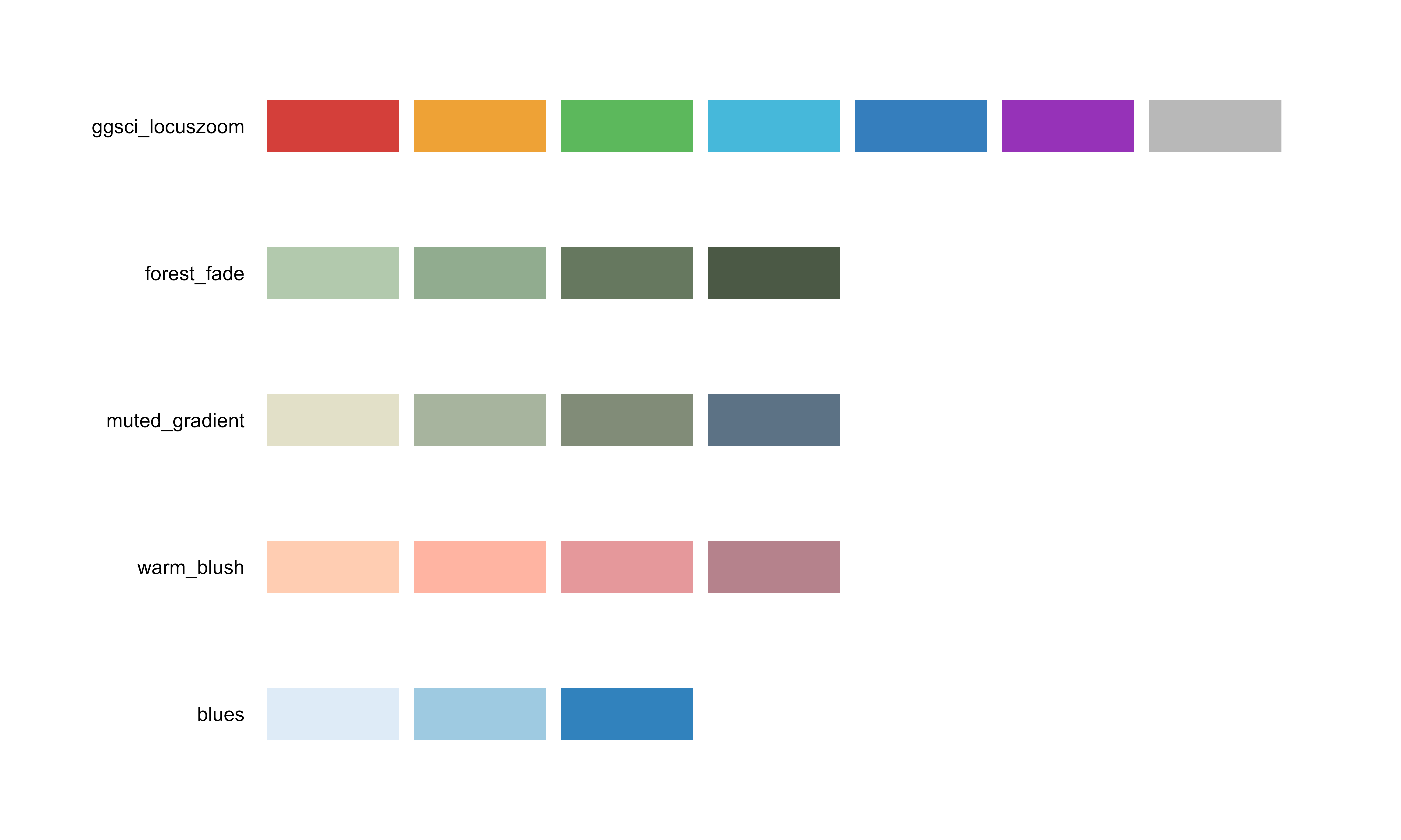
Complete gallery of all available palettes organized by type
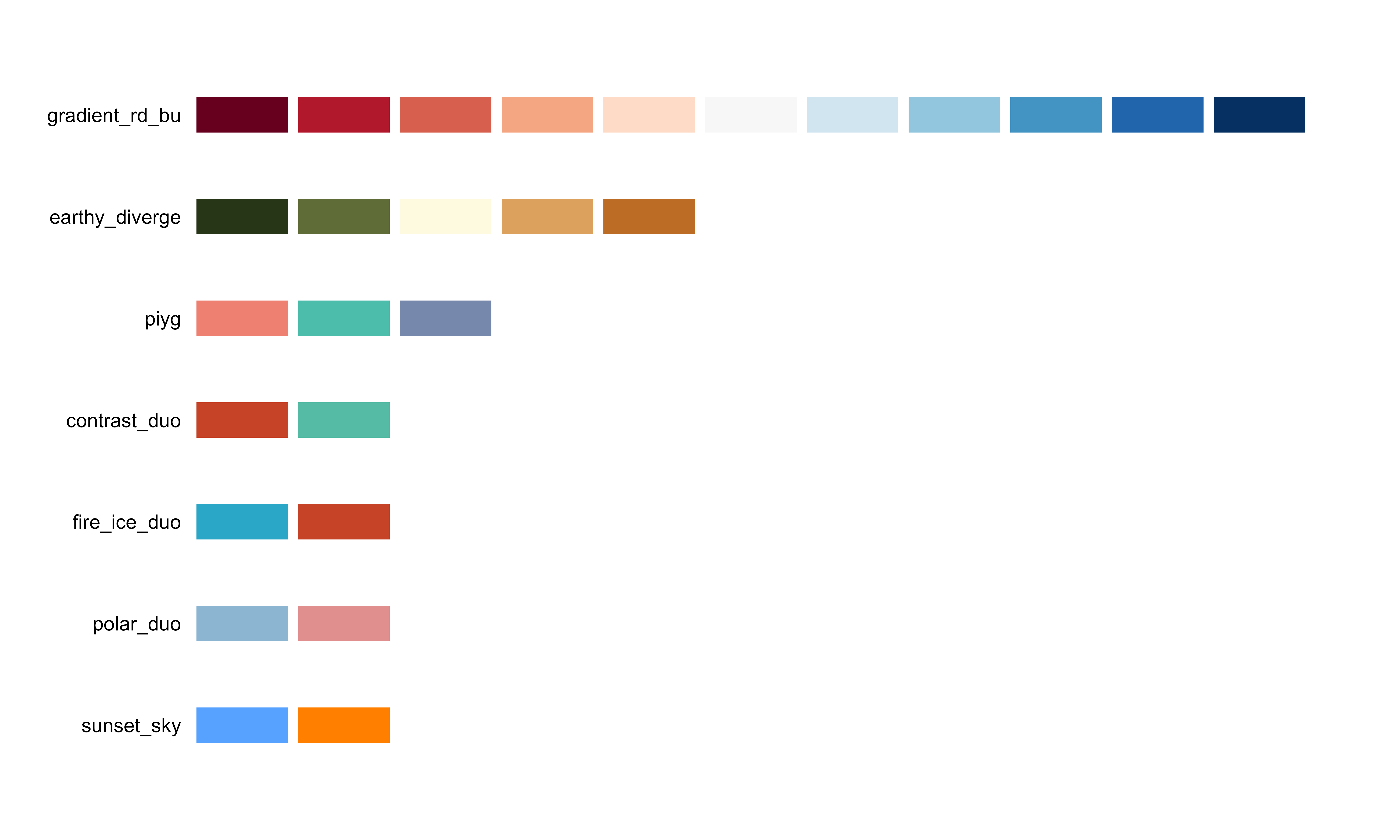
Complete gallery of all available palettes organized by type
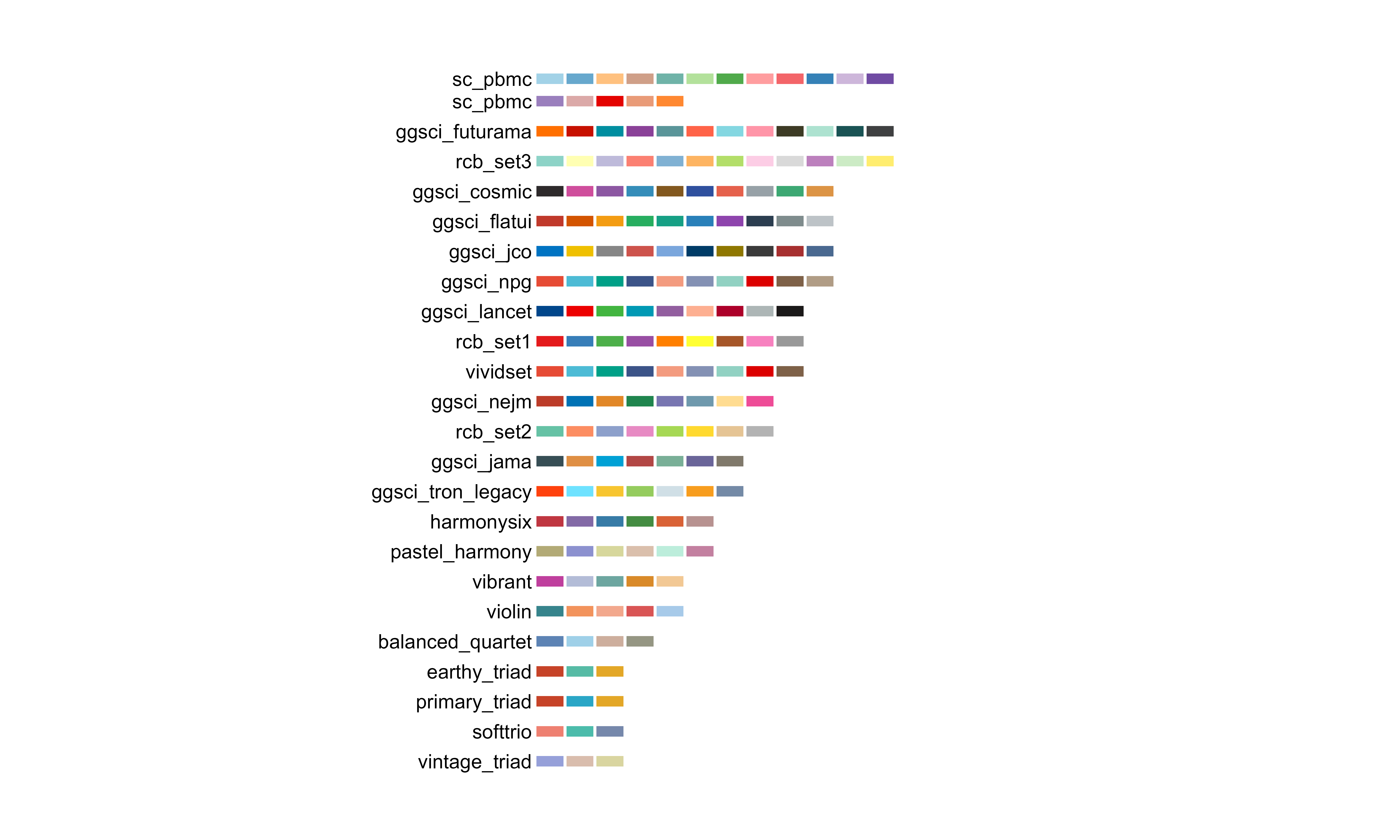
Complete gallery of all available palettes organized by type
2. Retrieve Palettes
Basic Retrieval
# Specify type explicitly for clarity
vivid_colors <- get_palette("qual_vivid", type = "qualitative")
cat("qual_vivid palette:\n")
#> qual_vivid palette:
print(vivid_colors)
#> [1] "#E64B35" "#4DBBD5" "#00A087" "#3C5488" "#F39B7F" "#8491B4" "#91D1C2"
#> [8] "#DC0000" "#7E6148"

# Get specific number of colors
blues_3 <- get_palette("seq_blues", type = "sequential", n = 3)
cat("\nseq_blues (3 colors):\n")
#>
#> seq_blues (3 colors):
print(blues_3)
#> [1] "#deebf7" "#9ecae1" "#3182bd"

# Get all available colors (omit n parameter)
blues_all <- get_palette("seq_blues", type = "sequential")
cat("\nseq_blues (all", length(blues_all), "colors):\n")
#>
#> seq_blues (all 3 colors):
print(blues_all)
#> [1] "#deebf7" "#9ecae1" "#3182bd"
Preview Palettes
# Save current par settings
oldpar <- par(no.readonly = TRUE)

# Preview different palette types
par(mfrow = c(2, 2), mar = c(3, 1, 2, 1))

# Qualitative
preview_palette("qual_vivid", type = "qualitative")
title("Qualitative: qual_vivid", cex.main = 1, font.main = 1)

# Sequential
preview_palette("seq_blues", type = "sequential")
title("Sequential: seq_blues", cex.main = 1, font.main = 1)

# Sequential - Another
preview_palette("seq_forest", type = "sequential")
title("Sequential: seq_forest", cex.main = 1, font.main = 1)

# Diverging
preview_palette("div_fireice", type = "diverging")
title("Diverging: div_fireice", cex.main = 1, font.main = 1)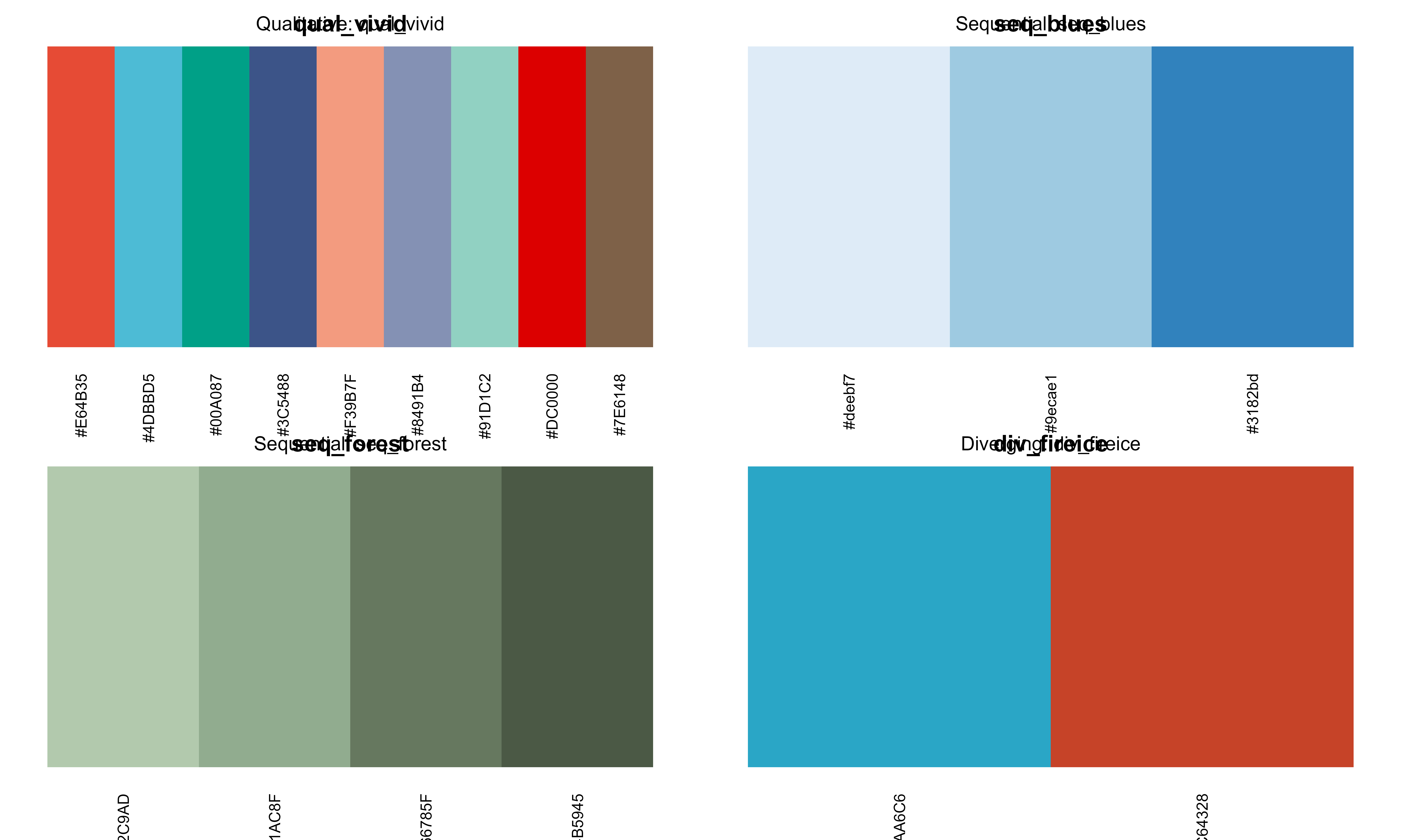
Preview of different palette types with color swatches
# Restore par settings
par(oldpar)
3. Create Custom Palettes
Step-by-Step Creation
# Step 1: Determine palette type
# Is your data continuous (sequential),
# categorical (qualitative), or centered (diverging)?

# Step 2: Define colors
ocean_colors <- c("#006BA4", "#FF7F0E", "#2CA02C", "#D62728", "#9467BD")

# Step 3: Create palette with proper naming
create_palette(
  name = "qual_ocean",  # Follow type_name_source convention
  type = "qualitative",
  colors = ocean_colors,
  color_dir = system.file("extdata", "palettes", package = "evanverse")
)

# Step 4: Compile palettes.rds (see next section)
Naming Your Custom Palette
# ✅ CORRECT naming
create_palette(
  name = "qual_custom",      # type_name
  name = "seq_thermal",      # for sequential
  name = "div_warmcool",     # for diverging
  name = "qual_nejm_g"       # if adapted from ggsci
)

# ❌ INCORRECT naming
create_palette(
  name = "MyPalette",        # Missing type, capital letters
  name = "custom.colors",    # Dot separator
  name = "palette_12"        # Number suffix
)
Color Utilities
# Convert between HEX and RGB
hex_colors <- c("#FF6B6B", "#4ECDC4", "#45B7D1")

# HEX to RGB
rgb_matrix <- hex2rgb(hex_colors)
cat("HEX to RGB:\n")
#> HEX to RGB:
print(rgb_matrix)
#> $`#FF6B6B`
#>   r   g   b
#> 255 107 107
#>
#> $`#4ECDC4`
#>   r   g   b
#>  78 205 196
#>
#> $`#45B7D1`
#>   r   g   b
#>  69 183 209

# RGB to HEX
hex_back <- rgb2hex(rgb_matrix)
cat("\nRGB to HEX:\n")
#>
#> RGB to HEX:
cat(paste(hex_back, collapse = ", "), "\n")
#> #FF6B6B, #4ECDC4, #45B7D1
4. Compile Palettes
After creating or modifying palette JSON files, compile them into the fast-loading RDS format:
# Compile all palettes from JSON to palettes.rds
compile_palettes(
  palettes_dir = system.file("extdata", "palettes", package = "evanverse"),
  output_rds = system.file("extdata", "palettes.rds", package = "evanverse")
)

# Test the new palette
get_palette("qual_ocean")
preview_palette("qual_ocean", type = "qualitative")Practical Applications
Qualitative: Categorical Data
# Sample categorical data
set.seed(123)
category_data <- data.frame(
  Group = rep(LETTERS[1:5], each = 20),
  Value = c(rnorm(20, 10, 2), rnorm(20, 15, 3), rnorm(20, 12, 2.5),
            rnorm(20, 18, 4), rnorm(20, 8, 1.5))
)

# Use qualitative palette
qual_colors <- get_palette("qual_vivid", type = "qualitative", n = 5)

ggplot(category_data, aes(x = Group, y = Value, fill = Group)) +
  geom_boxplot(alpha = 0.8, outlier.alpha = 0.6) +
  scale_fill_manual(values = qual_colors) +
  labs(
    title = "Qualitative Palette: Group Comparison",
    subtitle = "Using qual_vivid for categorical groups",
    x = "Experimental Group",
    y = "Measured Value"
  ) +
  theme_minimal() +
  theme(legend.position = "none")
Qualitative palette for categorical group comparison
Sequential: Continuous Data
# Generate expression matrix
set.seed(456)
genes <- paste0("Gene", 1:10)
samples <- paste0("S", 1:8)
expr_matrix <- matrix(rnorm(80, mean = 5, sd = 2), nrow = 10)
rownames(expr_matrix) <- genes
colnames(expr_matrix) <- samples

# Convert to long format
expr_long <- expand.grid(Gene = genes, Sample = samples)
expr_long$Expression <- as.vector(expr_matrix)

# Use sequential palette
seq_colors <- get_palette("seq_mobility", type = "sequential")

ggplot(expr_long, aes(x = Sample, y = Gene, fill = Expression)) +
  geom_tile(color = "white", linewidth = 0.5) +
  scale_fill_gradientn(
    colors = seq_colors,
    name = "Expression"
  ) +
  labs(
    title = "Sequential Palette: Gene Expression Heatmap",
    subtitle = "Using seq_blues for continuous expression data"
  ) +
  theme_minimal() +
  theme(panel.grid = element_blank())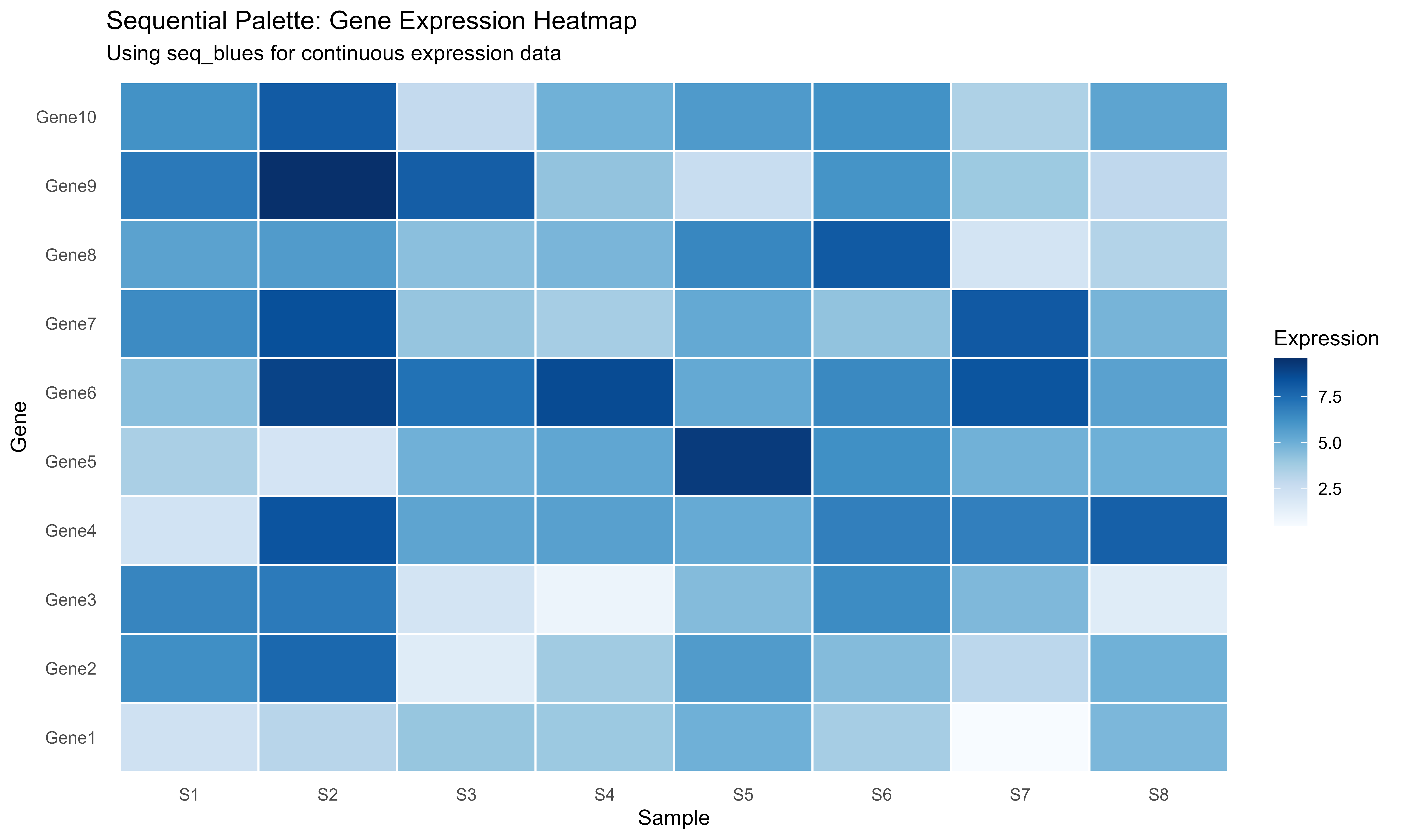
Sequential palette for continuous heatmap data
Diverging: Centered Data
# Generate fold change data
set.seed(789)
fc_data <- data.frame(
  Gene = paste0("Gene_", 1:20),
  LogFC = rnorm(20, 0, 1.2),
  Sample = rep(paste0("Sample_", 1:4), each = 5)
)

# Use diverging palette
div_colors <- get_palette("div_fireice", type = "diverging")

ggplot(fc_data, aes(x = Sample, y = Gene, fill = LogFC)) +
  geom_tile(color = "white", linewidth = 0.3) +
  scale_fill_gradientn(
    colors = div_colors,
    name = "Log2 FC",
    limits = c(-3, 3)
  ) +
  labs(
    title = "Diverging Palette: Fold Changes",
    subtitle = "Using div_fireice for centered data (zero midpoint)"
  ) +
  theme_minimal() +
  theme(panel.grid = element_blank())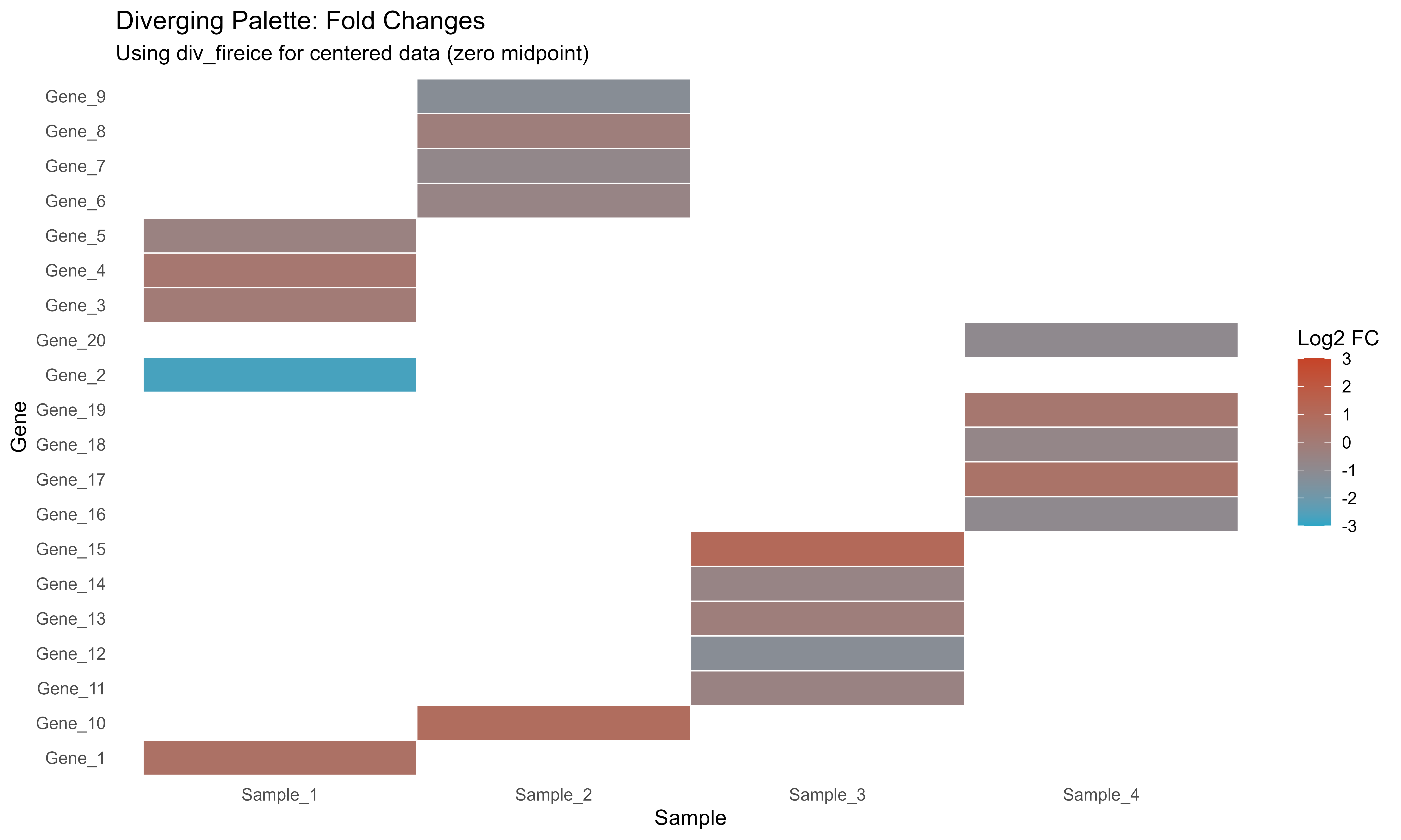
Diverging palette for fold change data
Bioinformatics Applications
Palette Selection Guide
By Data Type
Gene Expression - Sequential:
seq_blues, seq_forest for one-directional
intensity - Diverging: div_fireice, div_sunset
for fold changes
Single-Cell Data - Qualitative:
qual_pbmc_sc for cell types - Sequential:
seq_muted for UMAP/tSNE features
Pathway Analysis - Qualitative:
qual_vivid, qual_pastel for pathways -
Sequential: seq_blues for p-value gradients
Multi-omics - Qualitative: qual_vivid
for distinct data types - Avoid red/green for colorblind
accessibility
Multi-omics Example
# Simulate multi-omics data
set.seed(321)
omics_data <- data.frame(
  Sample = rep(paste0("P", 1:8), each = 3),
  DataType = rep(c("Transcriptome", "Proteome", "Metabolome"), 8),
  Intensity = c(
    rnorm(8, 100, 20),  # Transcriptome
    rnorm(8, 50, 15),   # Proteome
    rnorm(8, 25, 8)     # Metabolome
  ),
  Condition = rep(rep(c("Control", "Treatment"), each = 4), 3)
)

# Use qualitative palette for data types
omics_colors <- get_palette("qual_vivid", type = "qualitative", n = 3)
names(omics_colors) <- c("Transcriptome", "Proteome", "Metabolome")

ggplot(omics_data, aes(x = Sample, y = Intensity, fill = DataType)) +
  geom_bar(stat = "identity", position = "dodge", alpha = 0.85) +
  scale_fill_manual(values = omics_colors) +
  facet_wrap(~Condition, scales = "free_x") +
  labs(
    title = "Multi-omics Data Integration",
    subtitle = "Using qual_vivid to distinguish omics layers",
    x = "Patient Samples",
    y = "Normalized Intensity"
  ) +
  theme_minimal() +
  theme(
    axis.text.x = element_text(angle = 45, hjust = 1, size = 9),
    legend.position = "bottom"
  )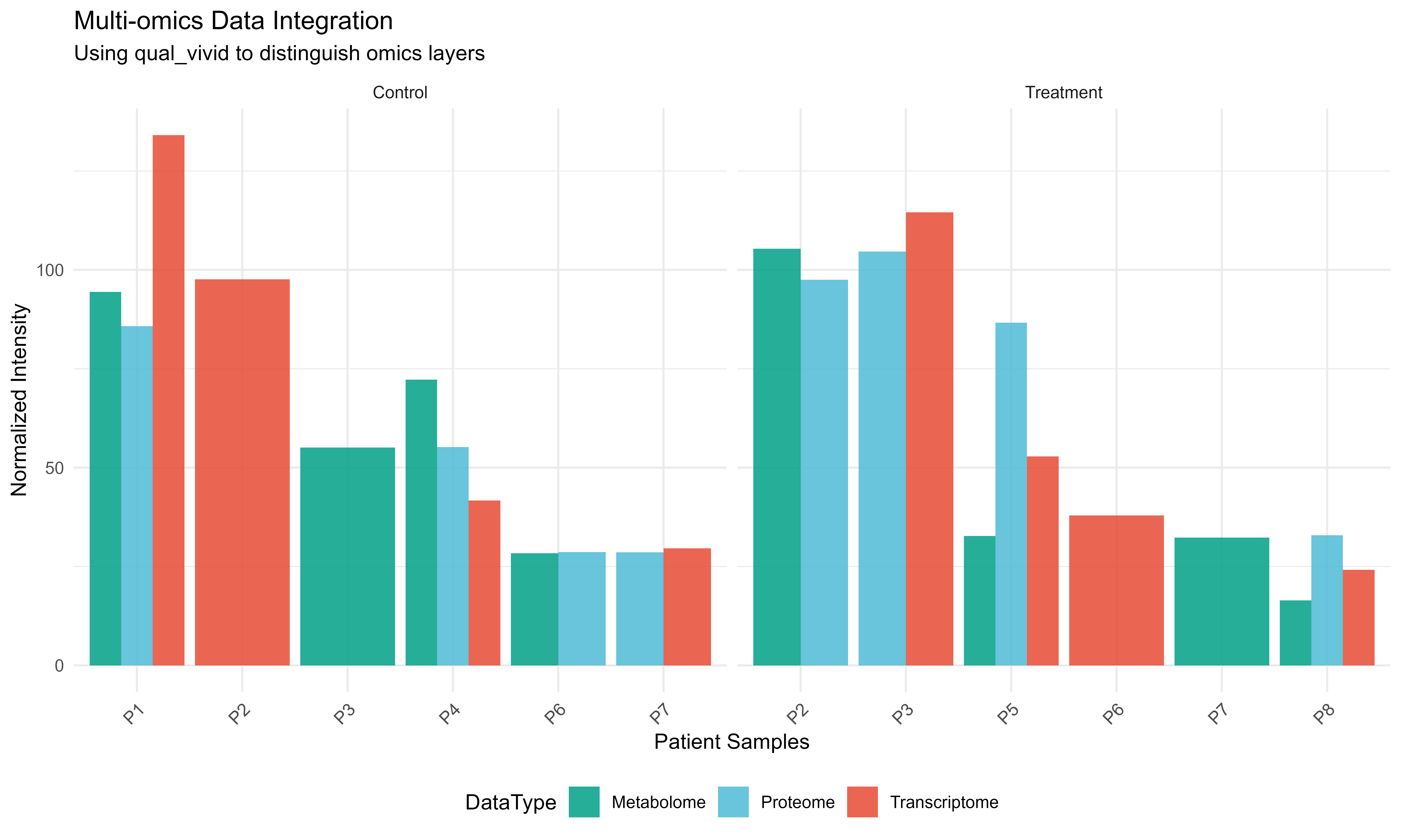
Multi-omics visualization with appropriate palette selection
Advanced Techniques
Color Interpolation
# Get base colors from qualitative palette
base_colors <- get_palette("qual_vivid", type = "qualitative", n = 3)

# Interpolate to create smooth gradient
custom_gradient <- colorRampPalette(base_colors[1:2])(10)

# Visualize the gradient
gradient_df <- data.frame(
  x = 1:10,
  y = rep(1, 10),
  color = custom_gradient
)

ggplot(gradient_df, aes(x = x, y = y, fill = color)) +
  geom_tile(height = 0.5, width = 0.9) +
  scale_fill_identity() +
  labs(
    title = "Custom Color Interpolation",
    subtitle = "Creating gradients from qualitative palette colors"
  ) +
  theme_void() +
  theme(plot.title = element_text(hjust = 0.5))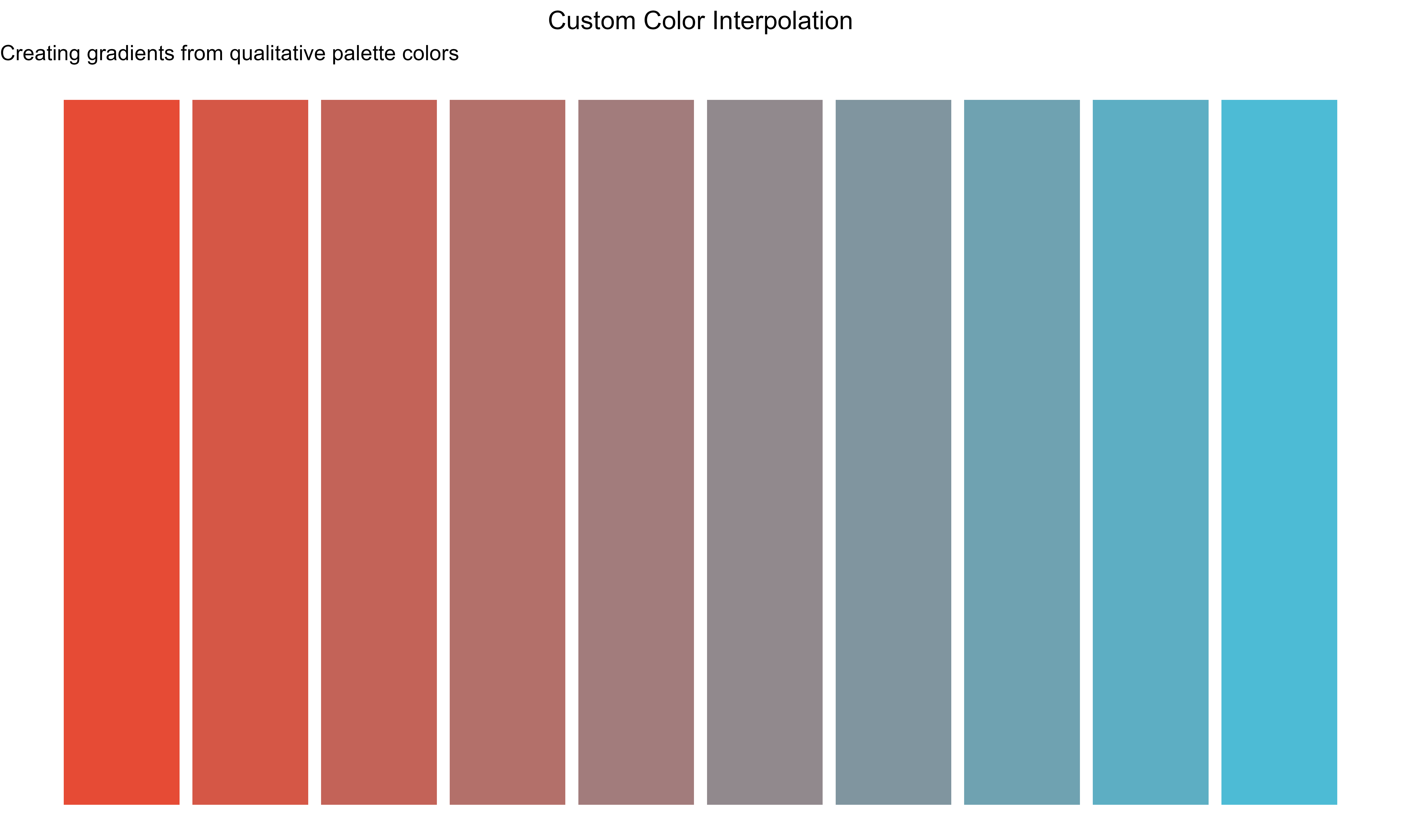
Creating custom gradients through color interpolation
Palette Combinations
# Combine palettes for complex visualizations
main_colors <- get_palette("qual_vivid", n = 4)
accent_color <- get_palette("div_fireice", n = 1)

# Use in multi-layer plots
ggplot(data) +
  geom_point(aes(color = group), size = 3) +
  geom_smooth(color = accent_color, linewidth = 1.5) +
  scale_color_manual(values = main_colors)
Best Practices
Accessibility Guidelines
Color Vision Deficiency - Test with colorblind simulators - Avoid red/green combinations alone - Use high contrast ratios (minimum 3:1) - Add texture/shape variations
Multi-Platform Compatibility - Test on different displays (mobile, print, projector) - Ensure sufficient color separation - Check grayscale conversion
Data Visualization - Match palette type to data type - Limit qualitative palettes to 8-10 categories - Use consistent colors across related plots - Reserve bright colors for emphasis
Performance Tips
# ✅ GOOD: Cache palette once
my_colors <- get_palette("qual_vivid", n = 5)
ggplot(data) + scale_fill_manual(values = my_colors)

# ❌ AVOID: Repeated calls
ggplot(data) + scale_fill_manual(values = get_palette("qual_vivid", n = 5))
Troubleshooting
Common Issues
Palette not found
# Check available palettes
list_palettes(type = "qualitative")
Not enough colors
# Check palette size
length(get_palette("qual_vivid"))

# Or use interpolation
colorRampPalette(get_palette("qual_vivid"))(20)
Colors don’t match
# Verify palette type
# Type is inferred from name prefix
get_palette("seq_blues")  # Automatically knows it's sequential
Custom palette not working
# Ensure you compiled after creation
compile_palettes(
  palettes_dir = system.file("extdata", "palettes", package = "evanverse"),
  output_rds = system.file("extdata", "palettes.rds", package = "evanverse")
)
Summary
Key Features
- 80+ curated palettes organized by type
-
Standardized naming (
type_name_sourceconvention) - Flexible workflow from creation to compilation to usage
- Scientific focus optimized for bioinformatics
- Publication-ready professional quality
Quick Reference
# Discover
list_palettes(type = "sequential")
bio_palette_gallery()

# Retrieve
get_palette("seq_blues")
preview_palette("qual_vivid", type = "qualitative")

# Create
create_palette(
  name = "qual_custom",
  type = "qualitative",
  colors = c("#E64B35", "#4DBBD5", "#00A087")
)

# Compile
compile_palettes(
  palettes_dir = system.file("extdata", "palettes", package = "evanverse"),
  output_rds = system.file("extdata", "palettes.rds", package = "evanverse")
)

# Utilities
hex2rgb("#FF6B6B")
rgb2hex(matrix(c(255, 107, 107), nrow = 1))
Related Documentation
-
Naming Convention:
vignette("palette-naming-convention")- Complete naming standards -
Package Guide:
vignette("get-started")- General evanverse overview -
Function Reference:
?get_palette,?create_palette,?compile_palettes
Document Version: 2.0 Last Updated: 2026-03-10 Status: Official Documentation