Publication-ready forest plot — plot

Produces a publication-ready forest plot with UKB-standard styling. The user supplies a data frame whose first column is the row label (item), plus any additional display columns (e.g. Cases/N). The gap column and the auto-formatted OR (95% CI) text column are inserted automatically at ci_column. Numeric p-value columns declared via p_cols are formatted in-place.

Usage

plot_forest(
  data,
  est,
  lower,
  upper,
  ci_column = 2L,
  ref_line = 1,
  xlim = NULL,
  ticks_at = NULL,
  arrow_lab = c("Lower risk", "Higher risk"),
  header = NULL,
  indent = NULL,
  bold_label = NULL,
  ci_col = "black",
  ci_sizes = 0.6,
  ci_Theight = 0.2,
  ci_digits = 2L,
  ci_sep = ", ",
  p_cols = NULL,
  p_digits = 3L,
  bold_p = TRUE,
  p_threshold = 0.05,
  align = NULL,
  background = "zebra",
  bg_col = "#F0F0F0",
  border = "three_line",
  border_width = 3,
  row_height = NULL,
  col_width = NULL,
  save = FALSE,
  dest = NULL,
  save_width = 20,
  save_height = NULL,
  theme = "default"
)

Arguments

data: data.frame. First column must be the label column (item). Additional columns are displayed as-is (character) or formatted if named in p_cols (must be numeric). Column order is preserved.
est: Numeric vector. Point estimates (NA = no CI drawn).
lower: Numeric vector. Lower CI bounds (same length as est).
upper: Numeric vector. Upper CI bounds (same length as est).
ci_column: Integer. Column position in the final rendered table where the gap/CI graphic is placed. Must be between 2 and ncol(data) + 1 (inclusive). Default: 2L.
ref_line: Numeric. Reference line. Default: 1 (HR/OR). Use 0 for beta coefficients.
xlim: Numeric vector of length 2. X-axis limits. NULL (default) uses c(0, 2).
ticks_at: Numeric vector. Tick positions. NULL (default) = 5 evenly spaced ticks across xlim.
arrow_lab: Character vector of length 2. Directional labels. Default: c("Lower risk", "Higher risk"). NULL = none.
header: Character vector of length ncol(data) + 2. Column header labels for the final rendered table (original columns + gap_ci + OR label). NULL (default) = use column names from data plus "gap_ci" and "OR (95% CI)". Pass "" for the gap column position.
indent: Integer vector (length = nrow(data)). Indentation level of the label column: each unit adds two leading spaces. Default: all zeros.
bold_label: Logical vector (length = nrow(data)). Which rows to bold in the label column. NULL (default) = auto-derive from indent: rows where indent == 0 are bolded (parent rows), indented sub-rows are plain.
ci_col: Character scalar or vector (length = nrow(data)). CI colour(s). NA rows are skipped automatically. Default: "black".
ci_sizes: Numeric. Point size. Default: 0.6.
ci_Theight: Numeric. CI cap height. Default: 0.2.
ci_digits: Integer. Decimal places for the auto-generated OR (95% CI) column. Default: 2L.
ci_sep: Character. Separator between lower and upper CI in the label, e.g. ", " or " - ". Default: ", ".
p_cols: Character vector. Names of numeric p-value columns in data. These are formatted to p_digits decimal places with "<0.001"-style clipping. NULL = none.
p_digits: Integer. Decimal places for p-value formatting. Default: 3L.
bold_p: TRUE (bold all non-NA p below p_threshold), FALSE (no bolding), or a logical vector (per-row control). Default: TRUE.
p_threshold: Numeric. P-value threshold for bolding when bold_p = TRUE. Default: 0.05.
align: Integer vector of length ncol(data) + 2. Alignment per column: -1 left, 0 centre, 1 right. Must cover all final columns (original + gap_ci + OR label). NULL = auto (column 1 left, all others centre).
background: Character. Row background style: "zebra", "bold_label" (shade rows where bold_label = TRUE), or "none". Default: "zebra".
bg_col: Character. Shading colour for backgrounds (scalar), or a per-row vector of length nrow(data) (overrides style). Default: "#F0F0F0".
border: Character. Border style: "three_line" or "none". Default: "three_line".
border_width: Numeric. Border line width(s). Scalar = all three lines same width; length-3 vector = top-of-header, bottom-of-header, bottom-of-body. Default: 3.
row_height: NULL (auto), numeric scalar, or numeric vector (length = total gtable rows including margins). Auto sets 8 / 12 / 10 / 15 mm for top / header / data / bottom respectively.
col_width: NULL (auto), numeric scalar, or numeric vector (length = total gtable columns). Auto rounds each default width up so the adjustment is in \([5, 10)\) mm.
save: Logical. Save output to files? Default: FALSE.
dest: Character. Destination file path (extension ignored; all four formats are saved). Required when save = TRUE.
save_width: Numeric. Output width in cm. Default: 20.
save_height: Numeric or NULL. Output height in cm. NULL = nrow(data) * 0.9 + 3.
theme: Character preset ("default") or a forestploter::forest_theme object. Default: "default".

Value

A forestploter plot object (gtable), returned invisibly. Display with plot() or grid::grid.draw().

Examples

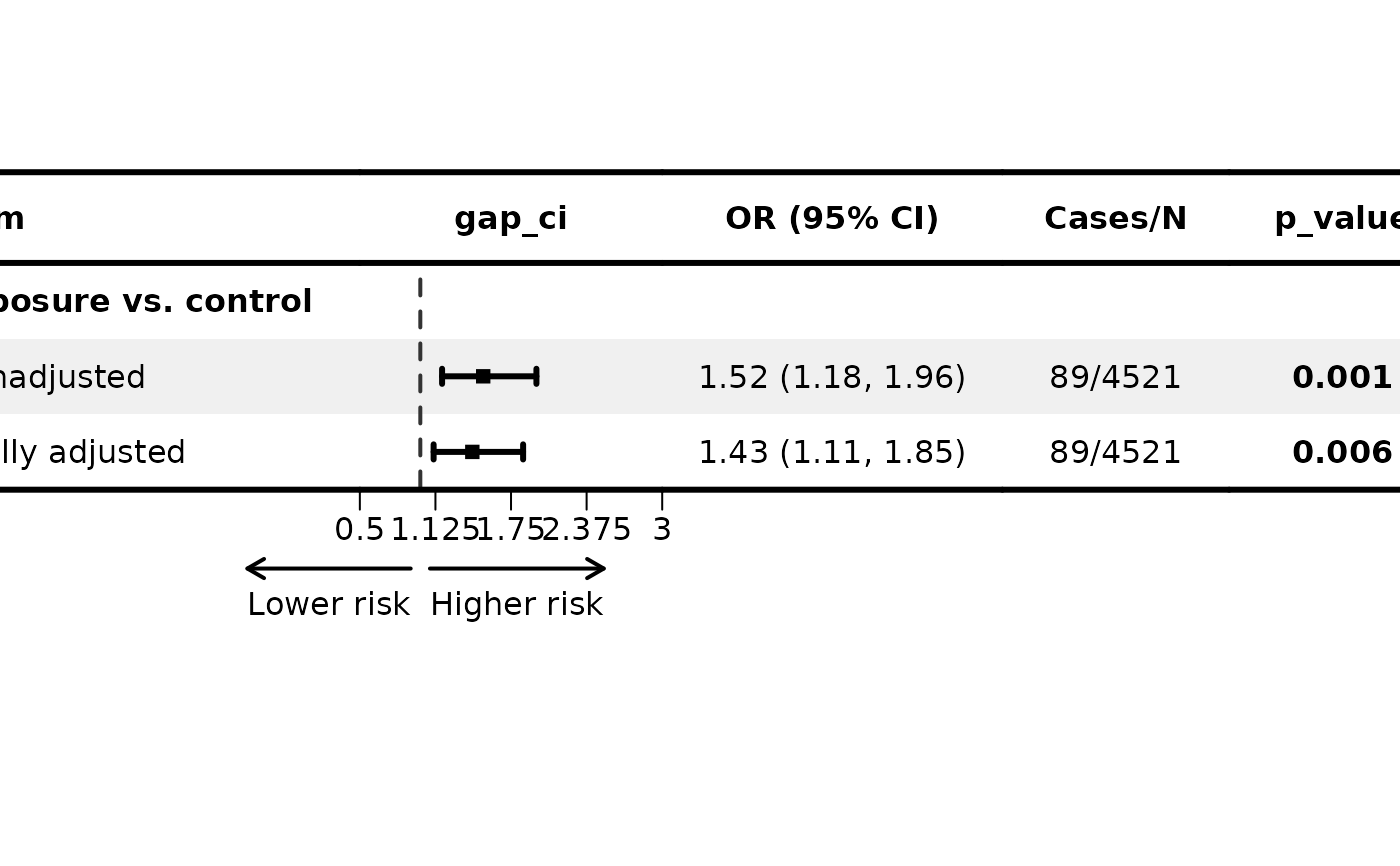
df <- data.frame(
  item      = c("Exposure vs. control", "Unadjusted", "Fully adjusted"),
  `Cases/N` = c("", "89/4521", "89/4521"),
  p_value   = c(NA_real_, 0.001, 0.006),
  check.names = FALSE
)

p <- plot_forest(
  data       = df,
  est        = c(NA, 1.52, 1.43),
  lower      = c(NA, 1.18, 1.11),
  upper      = c(NA, 1.96, 1.85),
  ci_column  = 2L,
  indent     = c(0L, 1L, 1L),
  bold_label = c(TRUE, FALSE, FALSE),
  p_cols     = "p_value",
  xlim       = c(0.5, 3.0)
)
plot(p)