Two-group comparison with automatic method selection

Performs a t-test or Wilcoxon test for exactly two groups, with automatic method selection based on normality when method = "auto". Always uses Welch's t-test for unpaired comparisons (no equal-variance assumption).

Usage

quick_ttest(
  data,
  group_col,
  value_col,
  method = c("auto", "t.test", "wilcox.test"),
  paired = FALSE,
  id_col = NULL,
  alternative = c("two.sided", "less", "greater"),
  alpha = 0.05
)

# S3 method for class 'quick_ttest_result'
plot(
  x,
  y = NULL,
  plot_type = c("boxplot", "violin", "both"),
  add_jitter = TRUE,
  point_size = 2,
  point_alpha = 0.6,
  show_p_value = TRUE,
  p_label = c("p.signif", "p.format"),
  palette = "qual_vivid",
  ...
)

Arguments

data: A data frame.
group_col: Character. Column name for the grouping variable (exactly 2 levels).
value_col: Character. Column name for the numeric response variable.
method: One of "auto" (default), "t.test", "wilcox.test".
paired: Logical. Paired test? Default FALSE. Requires id_col when TRUE.
id_col: Character. Column name for the pairing identifier. Required when paired = TRUE.
alternative: One of "two.sided" (default), "less", "greater".
alpha: Numeric. Significance level. Default 0.05.
x: A quick_ttest_result object from quick_ttest().
y: Ignored.
plot_type: One of "boxplot" (default), "violin", "both".
add_jitter: Logical. Add jittered points? Default TRUE.
point_size: Numeric. Jitter point size. Default 2.
point_alpha: Numeric. Jitter point transparency (0-1). Default 0.6.
show_p_value: Logical. Annotate plot with p-value? Default TRUE.
p_label: One of "p.signif" (stars, default) or "p.format" (numeric).
palette: evanverse palette name. Default "qual_vivid". NULL uses ggplot2 defaults.
...: Additional arguments passed to the internal plotting backend.

Value

An object of class "quick_ttest_result" (invisibly) containing:

test_result: An htest object from the test
method_used: Character: "t.test" or "wilcox.test"
descriptive_stats: Per-group summary data frame
normality_tests: Shapiro-Wilk results (auto mode only); NULL when method is forced
params: List of input parameters
data: Cleaned data frame used for the test (for plot() method)

Use print(result) for a one-line summary, summary(result) for full details, and plot(result) for a comparison plot.

Details

Auto method selection logic:

\(n \ge 100\): t-test (CLT applies; Shapiro-Wilk unreliable at large n)
\(30 \le n < 100\): Shapiro-Wilk at \(p < 0.01\) threshold
\(n < 30\): Shapiro-Wilk at \(p < 0.05\) threshold

Examples

set.seed(42)
df <- data.frame(
  group = rep(c("A", "B"), each = 30),
  value = c(rnorm(30, 5), rnorm(30, 6))
)
result <- quick_ttest(df, group_col = "group", value_col = "value")
print(result)
#> t.test | p = 0.0089* | A n=30, B n=30
summary(result)
#> 
#> ── Two-group Comparison ────────────────────────────────────────────────────────
#> 
#> ── Parameters ──
#> 
#> Test: Welch two-sample t-test
#> Direction: A - B
#> Alternative: two.sided
#> alpha: 0.050
#> Paired: FALSE
#> 
#> ── Result ──
#> 
#> ✔ p = 0.0089  (significant at alpha = 0.05)
#> 
#> 
#> 	Welch Two Sample t-test
#> 
#> data:  value by group
#> t = -2.7096, df = 56.249, p-value = 0.008913
#> alternative hypothesis: true difference in means between group A and group B is not equal to 0
#> 95 percent confidence interval:
#>  -1.4079331 -0.2110762
#> sample estimates:
#> mean in group A mean in group B 
#>        5.068587        5.878091 
#> 
#> 
#> ── Descriptive statistics ──
#> 
#> # A tibble: 2 × 7
#>   group     n  mean    sd median   min   max
#>   <fct> <int> <dbl> <dbl>  <dbl> <dbl> <dbl>
#> 1 A        30  5.07  1.26   4.90  2.34  7.29
#> 2 B        30  5.88  1.05   6.15  3.01  7.58
#> ── Normality (Shapiro-Wilk) ──
#> 
#> A: n = 30, p = 0.350
#> B: n = 30, p = 0.064
#> → Medium samples (min n = 30). Data reasonably normal (all Shapiro p ≥ 0.01).
#> 
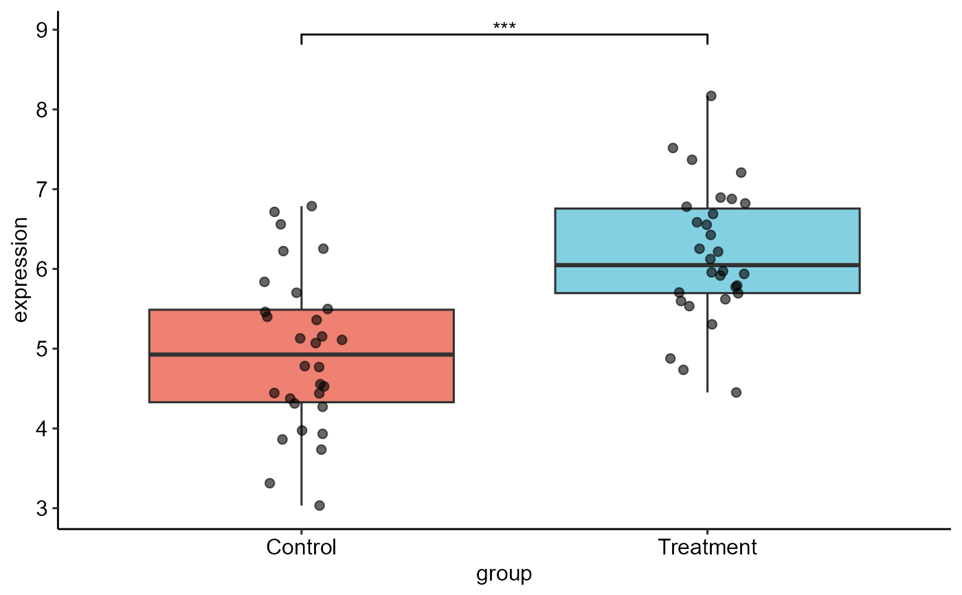
plot(result)