Perform correlation analysis with automatic p-value calculation and publication-ready heatmap visualization. Supports multiple correlation methods and significance testing with optional multiple testing correction.
Usage
quick_cor(
data,
vars = NULL,
method = c("pearson", "spearman", "kendall"),
use = "pairwise.complete.obs",
p_adjust_method = c("none", "holm", "hochberg", "hommel", "bonferroni", "BH", "BY",
"fdr"),
sig_level = c(0.001, 0.01, 0.05),
type = c("full", "upper", "lower"),
show_coef = FALSE,
show_sig = TRUE,
hc_order = TRUE,
hc_method = "complete",
palette = "gradient_rd_bu",
lab_size = 3,
title = NULL,
show_axis_x = TRUE,
show_axis_y = TRUE,
axis_x_angle = 45,
axis_y_angle = 0,
axis_text_size = 10,
verbose = TRUE,
...
)Arguments
- data
A data frame containing numeric variables.
- vars
Optional character vector specifying which variables to include. If
NULL(default), all numeric columns will be used.- method
Character. Correlation method: "pearson" (default), "spearman", or "kendall".
- use
Character. Method for handling missing values, passed to
cor(). Default is "pairwise.complete.obs". Other options: "everything", "all.obs", "complete.obs", "na.or.complete".- p_adjust_method
Character. Method for p-value adjustment for multiple testing. Default is "none". Options: "holm", "hochberg", "hommel", "bonferroni", "BH", "BY", "fdr", "none". See
p.adjust.- sig_level
Numeric vector. Significance levels for star annotations. Default is
c(0.001, 0.01, 0.05)corresponding to ***, **, *.- type
Character. Type of heatmap: "full" (default), "upper", or "lower".
- show_coef
Logical. Display correlation coefficients on the heatmap? Default is
FALSE.- show_sig
Logical. Display significance stars on the heatmap? Default is
TRUE.- hc_order
Logical. Reorder variables using hierarchical clustering? Default is
TRUE.- hc_method
Character. Hierarchical clustering method if
hc_order = TRUE. Default is "complete". Seehclust.- palette
Character. Color palette name from evanverse palettes. Default is "gradient_rd_bu" (diverging Red-Blue palette, recommended for correlation matrices). Set to
NULLto use ggplot2 defaults. Other diverging options: "piyg", "earthy_diverge", "fire_ice_duo".- lab_size
Numeric. Size of coefficient labels if
show_coef = TRUE. Default is 3.- title
Character. Plot title. Default is
NULL(no title).- show_axis_x
Logical. Display x-axis labels? Default is
TRUE.- show_axis_y
Logical. Display y-axis labels? Default is
TRUE.- axis_x_angle
Numeric. Rotation angle for x-axis labels in degrees. Default is 45. Common values: 0 (horizontal), 45 (diagonal), 90 (vertical).
- axis_y_angle
Numeric. Rotation angle for y-axis labels in degrees. Default is 0 (horizontal).
- axis_text_size
Numeric. Font size for axis labels. Default is 10.
- verbose
Logical. Print diagnostic messages? Default is
TRUE.- ...
Additional arguments (currently unused, reserved for future extensions).
Value
An object of class quick_cor_result containing:
- plot
A ggplot object with the correlation heatmap
- cor_matrix
Correlation coefficient matrix
- p_matrix
P-value matrix (unadjusted)
- p_adjusted
Adjusted p-value matrix (if p_adjust_method != "none")
- method_used
Correlation method used
- significant_pairs
Data frame of significant correlation pairs
- descriptive_stats
Descriptive statistics for each variable
- parameters
List of analysis parameters
- timestamp
POSIXct timestamp of analysis
Details
"Quick" means easy to use, not simplified or inaccurate.
This function performs complete correlation analysis with proper statistical testing:
Correlation Methods
Pearson: Measures linear relationships, assumes normality
Spearman: Rank-based, robust to outliers and non-normality
Kendall: Rank-based, better for small samples or many ties
P-value Calculation
P-values are calculated for each pairwise correlation. The function
automatically uses psych::corr.test() if the psych package
is installed, which provides significantly faster computation (10-100x speedup
for large matrices) compared to the base R stats::cor.test() loop.
If psych is not available, the function gracefully falls back to the
base R implementation.
For large correlation matrices with many tests, consider using
p_adjust_method to control for multiple testing (e.g., "bonferroni"
or "fdr").
Performance tip: Install the psych package for faster
p-value computation:
install.packages("psych")
Important Notes
Numeric variables only: The function automatically selects numeric columns or uses the variables specified in
vars.Constant variables: Variables with zero variance are automatically removed with a warning.
Sample size: The function will warn if sample sizes are very small (n < 5) after removing missing values.
Missing values: Handled according to the
useparameter. "pairwise.complete.obs" is recommended for optimal sample size usage.Optional dependencies: For optimal performance, install
psych(fast p-value computation) andggcorrplot(heatmap visualization). The function will work without them but may be slower or use fallback plotting.
Examples
# Example 1: Basic correlation analysis
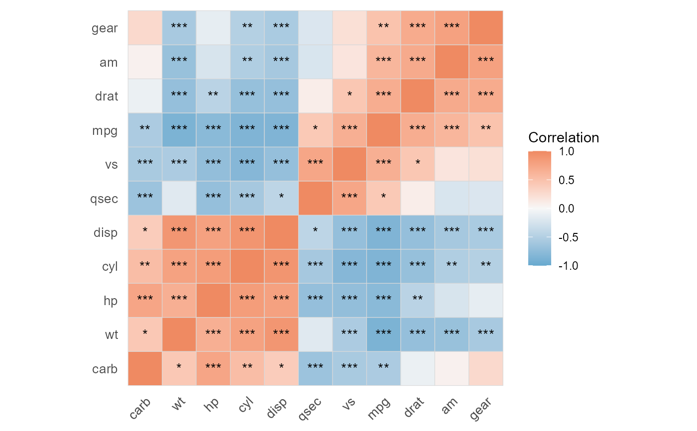
result <- quick_cor(mtcars)
#>
#> ── Data Preparation ──
#>
#> ℹ Automatically selected 11 numeric columns.
#>
#> ── Computing Correlations ──
#>
#> ℹ Found 44 significant correlations out of 55 tests
#> ! Found 1 pair with |r| > 0.9 (potential multicollinearity)
#>
#> ── Creating Heatmap ──
#>
#> ✔ Analysis complete!
print(result)
#>
#>
#> ── Quick Correlation Analysis Results ──
#>
#>
#> ℹ Method: pearson
#> ℹ Variables: 11
#> ℹ Significant pairs: 44
#>
#>
#> ── Top 5 Significant Correlations
#> var1 var2 correlation p_value
#> cyl disp 0.9020329 1.802838e-12
#> disp wt 0.8879799 1.222320e-11
#> mpg wt -0.8676594 1.293959e-10
#> mpg cyl -0.8521620 6.112687e-10
#> mpg disp -0.8475514 9.380327e-10
#>
#> Use `summary()` for detailed results.
# Example 2: Spearman correlation with specific variables
result <- quick_cor(
mtcars,
vars = c("mpg", "hp", "wt", "qsec"),
method = "spearman"
)
#>
#> ── Data Preparation ──
#>
#> ℹ Using 4 specified variables.
#>
#> ── Computing Correlations ──
#>
#> ℹ Found 5 significant correlations out of 6 tests
#>
#> ── Creating Heatmap ──
#>
#> ✔ Analysis complete!
# Example 3: Upper triangular with Bonferroni correction
result <- quick_cor(
iris,
type = "upper",
p_adjust_method = "bonferroni",
show_coef = TRUE
)
#> ! Both `show_coef` and `show_sig` are TRUE. Setting `show_sig` to FALSE to avoid overlapping labels.
#>
#> ── Data Preparation ──
#>
#> ℹ Automatically selected 4 numeric columns.
#>
#> ── Computing Correlations ──
#>
#> ℹ Applying bonferroni correction for multiple testing...
#> ℹ Found 5 significant correlations out of 6 tests
#> ! Found 1 pair with |r| > 0.9 (potential multicollinearity)
#>
#> ── Creating Heatmap ──
#>
#> ✔ Analysis complete!
# Example 4: Custom palette and title
result <- quick_cor(
mtcars,
palette = "gradient_rd_bu",
title = "Correlation Matrix of mtcars Dataset",
hc_order = TRUE
)
#>
#> ── Data Preparation ──
#>
#> ℹ Automatically selected 11 numeric columns.
#>
#> ── Computing Correlations ──
#>
#> ℹ Found 44 significant correlations out of 55 tests
#> ! Found 1 pair with |r| > 0.9 (potential multicollinearity)
#>
#> ── Creating Heatmap ──
#>
#> ✔ Analysis complete!
# Example 5: Customize axis labels
result <- quick_cor(
mtcars,
axis_x_angle = 90, # Vertical x-axis labels
axis_text_size = 12, # Larger text
show_axis_y = FALSE # Hide y-axis labels
)
#>
#> ── Data Preparation ──
#>
#> ℹ Automatically selected 11 numeric columns.
#>
#> ── Computing Correlations ──
#>
#> ℹ Found 44 significant correlations out of 55 tests
#> ! Found 1 pair with |r| > 0.9 (potential multicollinearity)
#>
#> ── Creating Heatmap ──
#>
#> ✔ Analysis complete!
# Access components
result$plot # ggplot object
result$cor_matrix # Correlation matrix
#> mpg cyl disp hp drat wt
#> mpg 1.0000000 -0.8521620 -0.8475514 -0.7761684 0.68117191 -0.8676594
#> cyl -0.8521620 1.0000000 0.9020329 0.8324475 -0.69993811 0.7824958
#> disp -0.8475514 0.9020329 1.0000000 0.7909486 -0.71021393 0.8879799
#> hp -0.7761684 0.8324475 0.7909486 1.0000000 -0.44875912 0.6587479
#> drat 0.6811719 -0.6999381 -0.7102139 -0.4487591 1.00000000 -0.7124406
#> wt -0.8676594 0.7824958 0.8879799 0.6587479 -0.71244065 1.0000000
#> qsec 0.4186840 -0.5912421 -0.4336979 -0.7082234 0.09120476 -0.1747159
#> vs 0.6640389 -0.8108118 -0.7104159 -0.7230967 0.44027846 -0.5549157
#> am 0.5998324 -0.5226070 -0.5912270 -0.2432043 0.71271113 -0.6924953
#> gear 0.4802848 -0.4926866 -0.5555692 -0.1257043 0.69961013 -0.5832870
#> carb -0.5509251 0.5269883 0.3949769 0.7498125 -0.09078980 0.4276059
#> qsec vs am gear carb
#> mpg 0.41868403 0.6640389 0.59983243 0.4802848 -0.55092507
#> cyl -0.59124207 -0.8108118 -0.52260705 -0.4926866 0.52698829
#> disp -0.43369788 -0.7104159 -0.59122704 -0.5555692 0.39497686
#> hp -0.70822339 -0.7230967 -0.24320426 -0.1257043 0.74981247
#> drat 0.09120476 0.4402785 0.71271113 0.6996101 -0.09078980
#> wt -0.17471588 -0.5549157 -0.69249526 -0.5832870 0.42760594
#> qsec 1.00000000 0.7445354 -0.22986086 -0.2126822 -0.65624923
#> vs 0.74453544 1.0000000 0.16834512 0.2060233 -0.56960714
#> am -0.22986086 0.1683451 1.00000000 0.7940588 0.05753435
#> gear -0.21268223 0.2060233 0.79405876 1.0000000 0.27407284
#> carb -0.65624923 -0.5696071 0.05753435 0.2740728 1.00000000
result$significant_pairs # Significant pairs
#> var1 var2 correlation p_value
#> 1 cyl disp 0.9020329 1.802838e-12
#> 2 disp wt 0.8879799 1.222320e-11
#> 3 mpg wt -0.8676594 1.293959e-10
#> 4 mpg cyl -0.8521620 6.112687e-10
#> 5 mpg disp -0.8475514 9.380327e-10
#> 6 cyl hp 0.8324475 3.477861e-09
#> 7 cyl vs -0.8108118 1.843018e-08
#> 8 am gear 0.7940588 5.834043e-08
#> 9 disp hp 0.7909486 7.142679e-08
#> 10 cyl wt 0.7824958 1.217567e-07
#> 11 mpg hp -0.7761684 1.787835e-07
#> 12 hp carb 0.7498125 7.827810e-07
#> 13 qsec vs 0.7445354 1.029669e-06
#> 14 hp vs -0.7230967 2.940896e-06
#> 15 drat am 0.7127111 4.726790e-06
#> 16 drat wt -0.7124406 4.784260e-06
#> 17 disp vs -0.7104159 5.235012e-06
#> 18 disp drat -0.7102139 5.282022e-06
#> 19 hp qsec -0.7082234 5.766253e-06
#> 20 cyl drat -0.6999381 8.244636e-06
#> 21 drat gear 0.6996101 8.360110e-06
#> 22 wt am -0.6924953 1.125440e-05
#> 23 mpg drat 0.6811719 1.776240e-05
#> 24 mpg vs 0.6640389 3.415937e-05
#> 25 hp wt 0.6587479 4.145827e-05
#> 26 qsec carb -0.6562492 4.536949e-05
#> 27 mpg am 0.5998324 2.850207e-04
#> 28 cyl qsec -0.5912421 3.660533e-04
#> 29 disp am -0.5912270 3.662114e-04
#> 30 wt gear -0.5832870 4.586601e-04
#> 31 vs carb -0.5696071 6.670496e-04
#> 32 disp gear -0.5555692 9.635921e-04
#> 33 wt vs -0.5549157 9.798492e-04
#> 34 mpg carb -0.5509251 1.084446e-03
#> 35 cyl carb 0.5269883 1.942340e-03
#> 36 cyl am -0.5226070 2.151207e-03
#> 37 cyl gear -0.4926866 4.173297e-03
#> 38 mpg gear 0.4802848 5.400948e-03
#> 39 hp drat -0.4487591 9.988772e-03
#> 40 drat vs 0.4402785 1.167553e-02
#> 41 disp qsec -0.4336979 1.314404e-02
#> 42 wt carb 0.4276059 1.463861e-02
#> 43 mpg qsec 0.4186840 1.708199e-02
#> 44 disp carb 0.3949769 2.526789e-02
summary(result) # Detailed summary
#>
#>
#> ── Detailed Correlation Analysis Summary ──
#>
#>
#> ── Analysis Parameters
#> Correlation method: pearson
#> Missing value handling: pairwise.complete.obs
#> P-value adjustment: none
#> Number of variables: 11
#>
#>
#> ── Descriptive Statistics
#> variable n mean sd median min max
#> mpg 32 20.090625 6.0269481 19.200 10.400 33.900
#> cyl 32 6.187500 1.7859216 6.000 4.000 8.000
#> disp 32 230.721875 123.9386938 196.300 71.100 472.000
#> hp 32 146.687500 68.5628685 123.000 52.000 335.000
#> drat 32 3.596563 0.5346787 3.695 2.760 4.930
#> wt 32 3.217250 0.9784574 3.325 1.513 5.424
#> qsec 32 17.848750 1.7869432 17.710 14.500 22.900
#> vs 32 0.437500 0.5040161 0.000 0.000 1.000
#> am 32 0.406250 0.4989909 0.000 0.000 1.000
#> gear 32 3.687500 0.7378041 4.000 3.000 5.000
#> carb 32 2.812500 1.6152000 2.000 1.000 8.000
#>
#>
#> ── Correlation Summary
#> Min correlation: -0.868
#> Max correlation: 0.902
#> Mean |correlation|: 0.559
#>
#>
#> ── Significant Correlations
#> ℹ Significant pairs are based on unadjusted p-values
#> Significant pairs: 44 out of 55 tests
#>
#> All significant pairs:
#> var1 var2 correlation p_value
#> cyl disp 0.9020329 1.802838e-12
#> disp wt 0.8879799 1.222320e-11
#> mpg wt -0.8676594 1.293959e-10
#> mpg cyl -0.8521620 6.112687e-10
#> mpg disp -0.8475514 9.380327e-10
#> cyl hp 0.8324475 3.477861e-09
#> cyl vs -0.8108118 1.843018e-08
#> am gear 0.7940588 5.834043e-08
#> disp hp 0.7909486 7.142679e-08
#> cyl wt 0.7824958 1.217567e-07
#> mpg hp -0.7761684 1.787835e-07
#> hp carb 0.7498125 7.827810e-07
#> qsec vs 0.7445354 1.029669e-06
#> hp vs -0.7230967 2.940896e-06
#> drat am 0.7127111 4.726790e-06
#> drat wt -0.7124406 4.784260e-06
#> disp vs -0.7104159 5.235012e-06
#> disp drat -0.7102139 5.282022e-06
#> hp qsec -0.7082234 5.766253e-06
#> cyl drat -0.6999381 8.244636e-06
#> drat gear 0.6996101 8.360110e-06
#> wt am -0.6924953 1.125440e-05
#> mpg drat 0.6811719 1.776240e-05
#> mpg vs 0.6640389 3.415937e-05
#> hp wt 0.6587479 4.145827e-05
#> qsec carb -0.6562492 4.536949e-05
#> mpg am 0.5998324 2.850207e-04
#> cyl qsec -0.5912421 3.660533e-04
#> disp am -0.5912270 3.662114e-04
#> wt gear -0.5832870 4.586601e-04
#> vs carb -0.5696071 6.670496e-04
#> disp gear -0.5555692 9.635921e-04
#> wt vs -0.5549157 9.798492e-04
#> mpg carb -0.5509251 1.084446e-03
#> cyl carb 0.5269883 1.942340e-03
#> cyl am -0.5226070 2.151207e-03
#> cyl gear -0.4926866 4.173297e-03
#> mpg gear 0.4802848 5.400948e-03
#> hp drat -0.4487591 9.988772e-03
#> drat vs 0.4402785 1.167553e-02
#> disp qsec -0.4336979 1.314404e-02
#> wt carb 0.4276059 1.463861e-02
#> mpg qsec 0.4186840 1.708199e-02
#> disp carb 0.3949769 2.526789e-02
#>
#> Analysis performed: 2025-11-25 13:57:14
