Stat

Overview

The stat module covers five common statistical workflows:

Task	Function
Power and sample-size planning	stat_power(), stat_n()
Two-group comparison	quick_ttest()
Multi-group comparison	quick_anova()
Categorical association	quick_chisq()
Correlation analysis	quick_cor()

library(evanverse)

The module is designed for quick, explicit statistical checks during analysis. It does not replace a full statistical modelling workflow; it gives small, repeatable wrappers around common tests with diagnostics, effect-size summaries, and plotting methods.

Power Planning

stat_power() computes achieved power from sample size and expected effect size.

power_res <- stat_power(
  n           = 30,
  effect_size = 0.5,
  test        = "t_two"
)

print(power_res)

✖ Power: 47.8%  (very low) | Two-sample t-test

n = 30 per group, effect size = 0.500, alpha = 0.050

With only 47.8% power, the study is unlikely to detect a true effect of size
0.50.

summary(power_res)

── Statistical Power Analysis ──────────────────────────────────────────────────

── Parameters ──

Test: Two-sample t-test

n: 30 per group

Effect size: 0.5000

alpha: 0.0500

Alternative: two.sided

── Result ──

✖ Power (1-beta): 47.79%  (very low)

── Interpretation ──

With only 47.8% power, the study is unlikely to detect a true effect of size
0.50.

── Recommendation ──

ℹ To reach 80% power, increase n from 30 to 64 per group.

plot(power_res)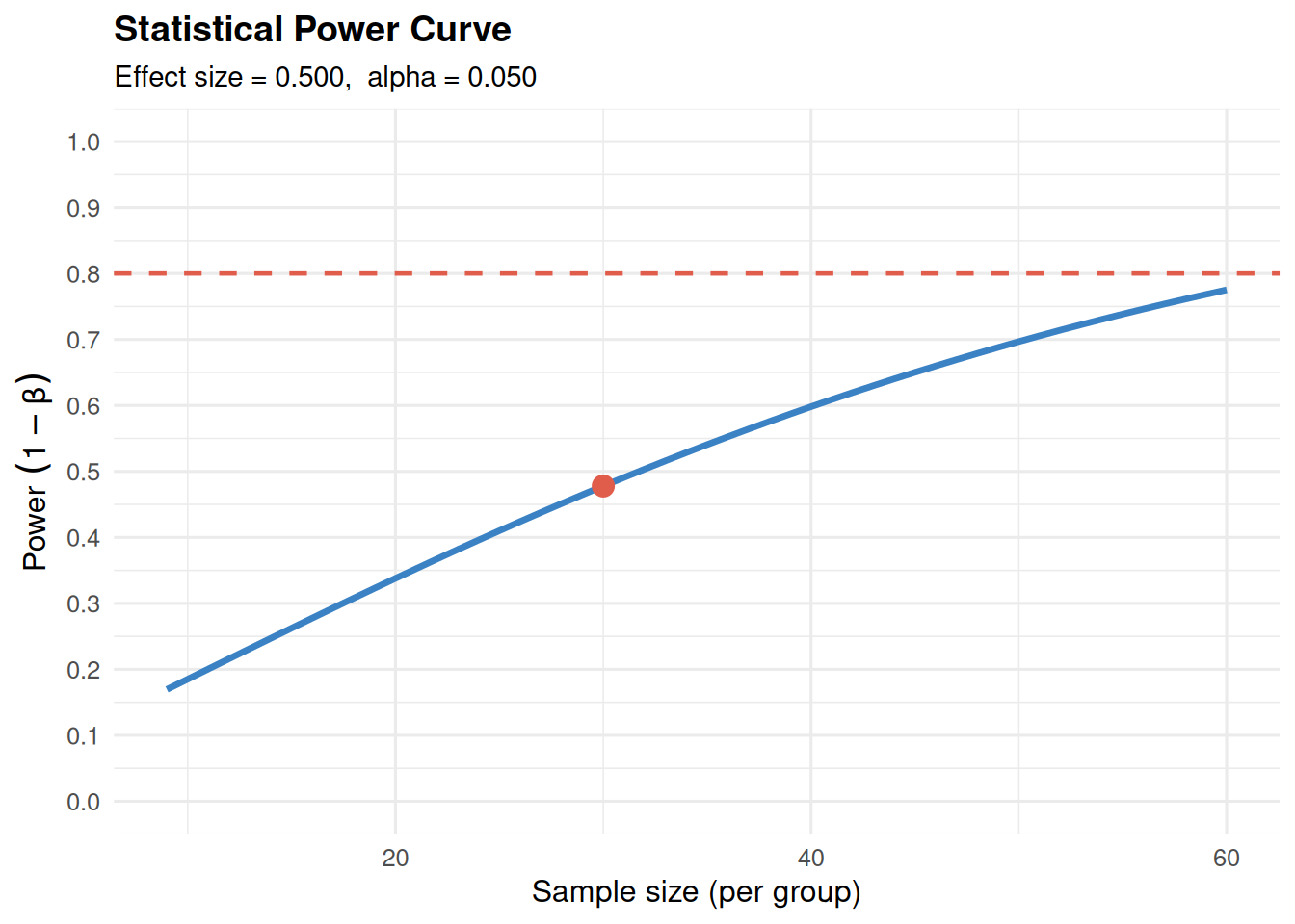

stat_n() computes the required sample size for a target power.

n_res <- stat_n(
  power       = 0.8,
  effect_size = 0.5,
  test        = "t_two"
)

print(n_res)

✔ n = 64 per group  (128 total) | Two-sample t-test

Target power = 80%, effect size = 0.500, alpha = 0.050

To detect an effect of size 0.50 with 80% power, recruit 64 subjects per group
(128 total).

plot(n_res)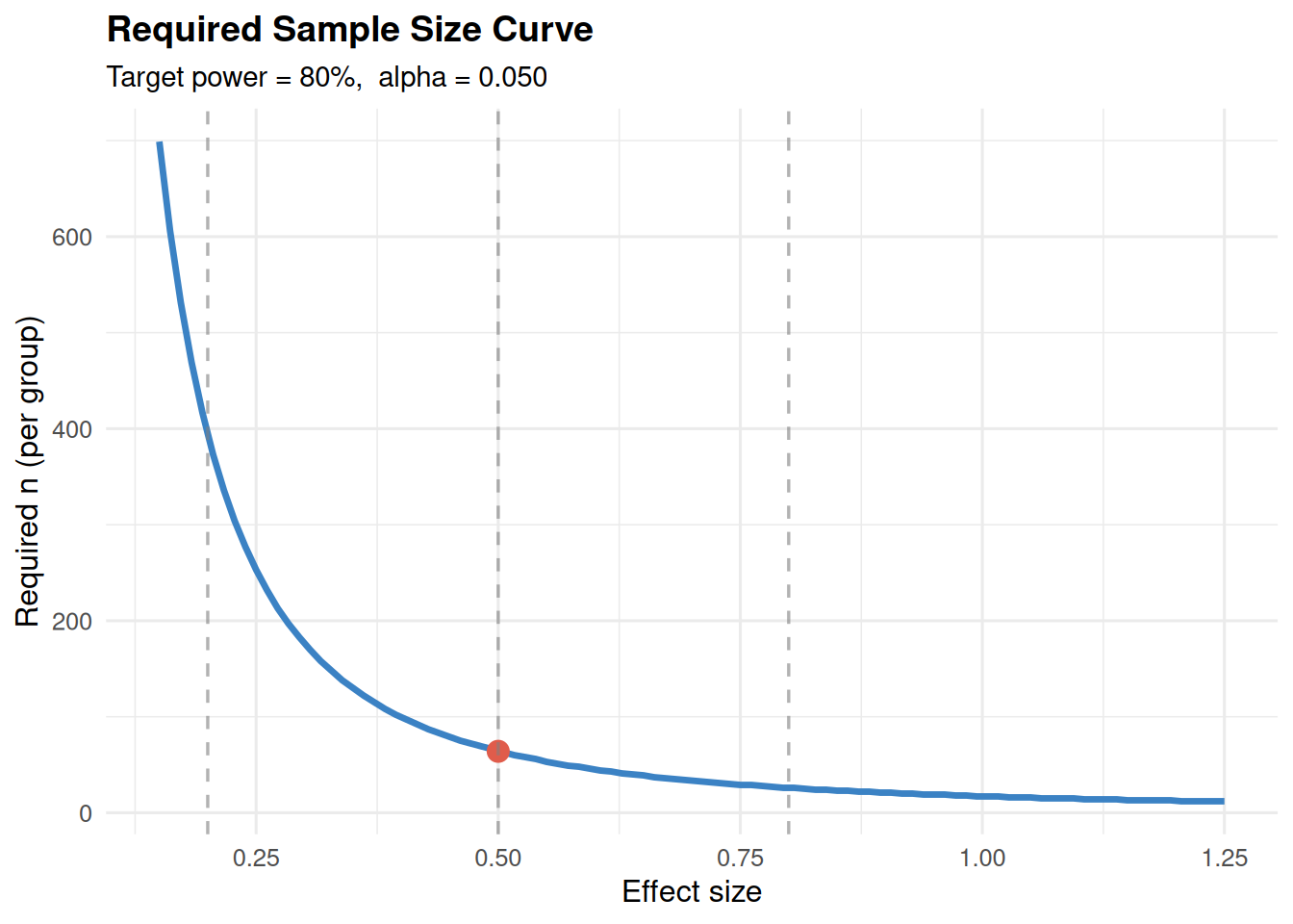

Supported test families share the same effect-size conventions:

test	Meaning	Effect size
"t_two"	Two-sample t-test	Cohen’s d
"t_one"	One-sample t-test	Cohen’s d
"t_paired"	Paired t-test	Cohen’s d
"anova"	One-way ANOVA	Cohen’s f
"proportion"	One-sample proportion test	Cohen’s h
"correlation"	Correlation test	Pearson r
"chisq"	Chi-square test	Cohen’s w

ANOVA requires k, the number of groups. Chi-square requires df, the degrees of freedom.

stat_power(n = 25, effect_size = 0.25, test = "anova", k = 3)
stat_n(power = 0.8, effect_size = 0.3, test = "chisq", df = 2)

Two-Group Comparison

quick_ttest() compares exactly two groups for a numeric outcome. With method = "auto", it checks normality and chooses between Welch’s t-test and a Wilcoxon test.

set.seed(42)
df <- data.frame(
  group = rep(c("A", "B"), each = 30),
  value = c(rnorm(30, 5), rnorm(30, 6))
)

tt <- quick_ttest(
  data      = df,
  group_col = "group",
  value_col = "value"
)

print(tt)

t.test | p = 0.0089* | A n=30, B n=30

summary(tt)

── Two-group Comparison ────────────────────────────────────────────────────────

── Parameters ──

Test: Welch two-sample t-test

Direction: A - B

Alternative: two.sided

alpha: 0.050

Paired: FALSE

── Result ──

✔ p = 0.0089  (significant at alpha = 0.05)

    Welch Two Sample t-test

data:  value by group
t = -2.7096, df = 56.249, p-value = 0.008913
alternative hypothesis: true difference in means between group A and group B is not equal to 0
95 percent confidence interval:
 -1.4079331 -0.2110762
sample estimates:
mean in group A mean in group B 
       5.068587        5.878091 

── Descriptive statistics ──

# A tibble: 2 × 7
  group     n  mean    sd median   min   max
  <fct> <int> <dbl> <dbl>  <dbl> <dbl> <dbl>
1 A        30  5.07  1.26   4.90  2.34  7.29
2 B        30  5.88  1.05   6.15  3.01  7.58

── Normality (Shapiro-Wilk) ──

A: n = 30, p = 0.350

B: n = 30, p = 0.064

→ Medium samples (min n = 30). Data reasonably normal (all Shapiro p ≥ 0.01).

plot(tt)

! Could not load palette "qual_vivid". Using ggplot2 defaults.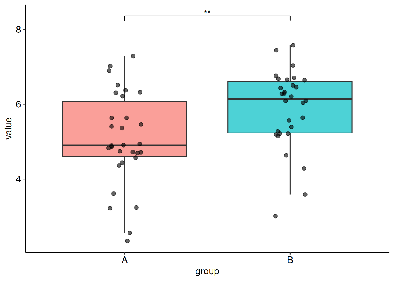

Independent comparisons use Welch’s t-test when the parametric path is selected. Paired comparisons require an ID column.

set.seed(7)
paired_df <- data.frame(
  id    = rep(seq_len(20), 2),
  group = rep(c("pre", "post"), each = 20),
  value = c(rnorm(20, 10, 2), rnorm(20, 11, 2))
)

quick_ttest(
  paired_df,
  group_col = "group",
  value_col = "value",
  paired    = TRUE,
  id_col    = "id"
)

Constant groups are allowed in the normality diagnostic path. Shapiro-Wilk is skipped for those groups, and the function continues with a clear message instead of failing inside stats::shapiro.test().

Multi-Group Comparison

quick_anova() compares two or more groups for a numeric outcome. With method = "auto", it uses group normality diagnostics and variance checks to choose among classical ANOVA, Welch ANOVA, and Kruskal-Wallis.

set.seed(123)
anova_df <- data.frame(
  group = rep(LETTERS[1:3], each = 40),
  value = rnorm(120, mean = rep(c(0, 0.5, 1.2), each = 40), sd = 1)
)

av <- quick_anova(
  anova_df,
  group_col = "group",
  value_col = "value"
)

print(av)

One-way ANOVA | p < 0.001* | A n=40, B n=40, C n=40

summary(av)

── One-way Comparison ──────────────────────────────────────────────────────────

── Parameters ──

Test: One-way ANOVA

alpha: 0.050

── Omnibus Test ──

✔ p < 0.001  (significant at alpha = 0.05)

eta_squared = 0.224, omega_squared = 0.210

             Df Sum Sq Mean Sq F value   Pr(>F)    
group         2  27.51  13.755   16.91 3.53e-07 ***
Residuals   117  95.14   0.813                     
---
Signif. codes:  0 '***' 0.001 '**' 0.01 '*' 0.05 '.' 0.1 ' ' 1

── Descriptive statistics ──

# A tibble: 3 × 7
  group     n   mean    sd median    min   max
  <fct> <int>  <dbl> <dbl>  <dbl>  <dbl> <dbl>
1 A        40 0.0452 0.898 0.0906 -1.97   1.79
2 B        40 0.493  0.960 0.437  -1.81   2.67
3 C        40 1.21   0.844 1.15   -0.468  3.39

── Normality (Shapiro-Wilk) ──

A: n = 40, p = 0.953

B: n = 40, p = 0.940

C: n = 40, p = 0.913

-> Medium samples (min n = 40). Data reasonably normal (all Shapiro p ≥ 0.01).

── Variance (Levene's test) ──

p = 0.854 | equal variances: TRUE

── Post-hoc (tukey) ──

# A tibble: 3 × 6
  group2 group1  diff     lwr   upr     `p adj`
  <chr>  <chr>  <dbl>   <dbl> <dbl>       <dbl>
1 B      A      0.448 -0.0306 0.927 0.0716     
2 C      A      1.16   0.684  1.64  0.000000201
3 C      B      0.715  0.236  1.19  0.00163    

plot(av)

! Could not load palette "qual_vivid". Using ggplot2 defaults.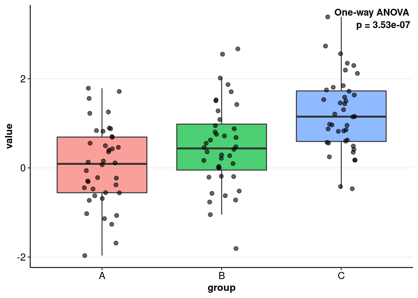

Post-hoc tests can be selected explicitly, or left on auto:

Omnibus method	Default post-hoc
anova	Tukey HSD
welch	Pairwise Welch t-tests, BH-adjusted
kruskal	Pairwise Wilcoxon tests, BH-adjusted

quick_anova(
  anova_df,
  group_col = "group",
  value_col = "value",
  method    = "anova",
  post_hoc  = "tukey"
)

Kruskal-Wallis results include epsilon-squared as an effect-size summary.

Categorical Association

quick_chisq() tests association between two categorical variables. The automatic method uses expected frequencies and table shape.

set.seed(123)
chisq_df <- data.frame(
  treatment = sample(c("A", "B", "C"), 100, replace = TRUE),
  response  = sample(c("Success", "Failure"), 100, replace = TRUE)
)

cs <- quick_chisq(
  chisq_df,
  x_col = "treatment",
  y_col = "response"
)

print(cs)

Chi-square test | p = 0.4128 | 3x2 | V = 0.133 (small)

summary(cs)

── Categorical Association Test ────────────────────────────────────────────────

── Parameters ──

Test: Chi-square test

Variables: treatment × response

Table size: 3x2

alpha: 0.050

── Result ──

ℹ p = 0.4128  (not significant at alpha = 0.05)

    Pearson's Chi-squared test

data:  cont_table
X-squared = 1.7694, df = 2, p-value = 0.4128

── Effect Size (Cramer's V) ──

V: 0.133

Interpretation: small

── Observed Frequencies ──

   
    Failure Success
  A      17      16
  B      21      11
  C      18      17

── Expected Frequencies ──

  Failure Success
A   18.48   14.52
B   17.92   14.08
C   19.60   15.40

── Pearson Residuals ──

   
    Failure Success
  A   -0.34    0.39
  B    0.73   -0.82
  C   -0.36    0.41

→ |residual| > 2 indicates significant deviation from independence

── Method Selection ──

Table size: 3x2

Total N: 100

Min expected freq: 14.08

Cells with freq < 5: 0

Decision: All expected frequencies adequate: using standard chi-square test

plot(cs)

! Failed to load palette 'qual_vivid': Palette "qual_vivid" not found in any type.. Using defaults.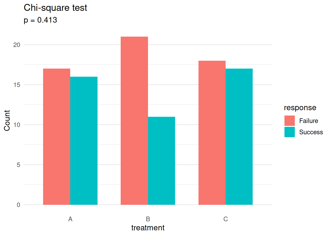

Method selection:

Case	Method
2x2 with expected frequency below 5	Fisher’s exact test
2x2 with moderate expected frequencies	Chi-square with Yates correction
Larger sparse tables	Chi-square with warning
Matched square table, explicit request	McNemar’s test

method = "mcnemar" is only for paired or matched categorical outcomes.

Correlation Analysis

quick_cor() computes a correlation matrix, p-values, optional p-value adjustment, and significant-pair summaries.

cor_res <- quick_cor(
  mtcars,
  vars = c("mpg", "hp", "wt", "qsec")
)

ℹ Found 5 significant pairs out of 6 tests.

print(cor_res)

pearson | 4 vars | 5/6 significant pairs (alpha = 0.05)

summary(cor_res)

── Correlation Analysis ────────────────────────────────────────────────────────

── Parameters ──

Method: pearson

Missing obs: pairwise.complete.obs

P-adjust: none

Variables: 4

alpha: 0.050

── Descriptive Statistics ──

 variable  n      mean         sd  median    min     max
      mpg 32  20.09062  6.0269481  19.200 10.400  33.900
       hp 32 146.68750 68.5628685 123.000 52.000 335.000
       wt 32   3.21725  0.9784574   3.325  1.513   5.424
     qsec 32  17.84875  1.7869432  17.710 14.500  22.900

── Correlation Summary ──

Min: -0.868

Max: 0.659

Mean |r|: 0.601

── Significant Pairs ──

ℹ Based on unadjusted p-values.

5 out of 6 pairs significant at alpha = 0.05

 var1 var2 correlation      p_value
  mpg   wt  -0.8676594 1.293959e-10
  mpg   hp  -0.7761684 1.787835e-07
   hp qsec  -0.7082234 5.766253e-06
   hp   wt   0.6587479 4.145827e-05
  mpg qsec   0.4186840 1.708199e-02

plot(cor_res, type = "upper", show_sig = TRUE)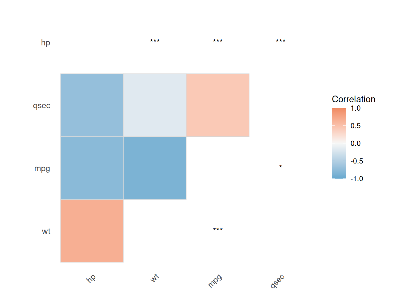

Use p_adjust_method when many pairs are tested.

quick_cor(
  mtcars,
  vars            = c("mpg", "hp", "wt", "qsec"),
  method          = "spearman",
  p_adjust_method = "BH"
)

ℹ Found 5 significant pairs out of 6 tests.

The use argument follows stats::cor() missing-value handling and is validated before the correlation is computed:

quick_cor(
  mtcars,
  use = "pairwise.complete.obs"
)

ℹ Found 44 significant pairs out of 55 tests.

! 1 pair with |r| > 0.9 (potential multicollinearity).

Valid choices are everything, all.obs, complete.obs, na.or.complete, and pairwise.complete.obs.

Design Notes

• stat_power() and stat_n() return the same S3 class, power_result, so print(), summary(), and plot() work consistently.
• quick_ttest() uses Welch’s t-test for independent parametric comparisons.
• Wilcoxon tests use exact = FALSE so common tied data do not create noisy exact-p-value warnings.
• Normality diagnostics skip constant groups instead of failing inside Shapiro-Wilk.
• quick_anova() still runs diagnostics when a method is forced, but the forced method is respected.
• quick_chisq() reports observed counts, expected frequencies, residuals when available, and Cramer’s V when a chi-square statistic exists.
• quick_cor() reports significant pairs based on adjusted p-values when p_adjust_method is not "none".
• Plot methods return the original result invisibly after printing the ggplot, matching the package’s reporting style.